
Page Contents
- Why Reach Beyond Symbolic Algebra?
- Choosing the Right Solver
- Closed-Form Integer Linear Systems and Curve Fitting
- Mixed-Integer Linear Programming with
scipy.optimize.milp - 1D Convex Optimisation:
minimize_scalarvs Median and Mean - Constraint Propagation and Stack Deduction
- AoC Examples
Why Reach Beyond Symbolic Algebra?
In Maths with SymPy, symbolic algebra gets you out of trouble fast when you just want to hand a handful of equations to Python and read off the answer. And for small square systems, SymPy works brilliantly.
Then Part 2 lands, and one of three things happens:
- The numbers explode to (10^{13}) or beyond, turning a nested
range(100)loop into heat-death-of-the-universe runtime — whilst running SymPy’s symbolic engine inside a loop of hundreds of puzzle inputs stretches a notebook cell from milliseconds to several seconds. - The system is underdetermined — more variables than equations, like 13 buttons wired to 10 counters — so
sympy.solve()shrugs and hands you free parameters instead of the smallest non-negative integer vector. - You don’t actually have equations at all, just noisy candidate sets (
dairymight bemxmxvkdorsqjhc) or unimodal cost functions where an integer lattice rounding slip changes the total by two.
That is the problem space where closed-form integer arithmetic, Mixed-Integer Linear Programming (scipy.optimize.milp), 1D convex search (scipy.optimize.minimize_scalar), and set-based constraint propagation shine. They stay deterministic, fast, and self-contained inside numpy, scipy, and the Python standard library — no external constraint solvers required.
Choosing the Right Solver
Before reaching for a heavyweight tool, match the mathematical shape of the puzzle to the lightest solver that preserves exact integer answers:
| Approach | Problem Shape | Integer Exactness | Typical AoC Runtime | Best AoC Fit |
|---|---|---|---|---|
Closed-Form Cramer’s Rule (divmod) |
Fixed small linear systems ((2 \times 2)) | Exact (arbitrary-precision int) |
Microseconds for hundreds of systems | 2024 Day 13 (Claw Contraption) |
Finite Differences / Fraction Fit |
Periodic growth sampled at 3 points | Exact (int or Fraction) |
Sub-millisecond once samples exist | 2023 Day 21 (Step Counter) |
sympy.solve |
Ad-hoc nonlinear or square symbolic equations | Exact symbolic rationals | Milliseconds per solve (hundreds of ms in loops) | 2023 Day 6, 2023 Day 24 |
scipy.optimize.milp |
Minimise (\mathbf{c}^T \mathbf{x}) subject to (A\mathbf{x} = \mathbf{b}), (\mathbf{x} \in \mathbb{Z}_{\ge 0}^n) | Exact after np.rint + matrix verify |
Milliseconds per machine | 2025 Day 10 (Factory Joltages) |
Median / Mean / minimize_scalar |
Smooth 1D convex or unimodal integer cost | Must check floor and ceil |
Sub-millisecond | 2021 Day 7 (Treachery of Whales) |
| Bipartite Constraint Propagation | 1-to-1 bijection from candidate sets | Exact by set elimination | Microseconds | 2020 Days 16 & 21, 2021 Day 8 |
Closed-Form Integer Linear Systems and Curve Fitting
Exact 2x2 Linear Systems with Cramer’s Rule
In 2024 Day 13 — Claw Contraption (2024 Notebook), each machine gives two buttons moving a claw by ((A_x, A_y)) and ((B_x, B_y)), and asks for non-negative integer presses ((a, b)) that land cleanly on ((P_x, P_y)) whilst minimising (3a + b):
\[a A_x + b B_x = P_x, \qquad a A_y + b B_y = P_y\]Notice there is actually nothing to “optimise” once the button vectors are linearly independent! Two equations in two unknowns have at most one solution. Let (\Delta = A_x B_y - A_y B_x). By Cramer’s rule:
\[a = \frac{P_x B_y - P_y B_x}{\Delta}, \qquad b = \frac{A_x P_y - A_y P_x}{\Delta}\]When Part 2 adds (10^{13}) to both prize coordinates, brute force dies instantly. SymPy solves it cleanly, yet even SymPy pays symbolic parsing overhead across hundreds of machines. Worse, a quick NumPy or plain-Python floating-point shortcut (a = num / det; if a % 1 == 0) risks precision drift at (10^{13})+ scales where IEEE 754 float64 only has 53 bits of significand precision (about (9 \times 10^{15})). Multiply two large terms together before dividing, and floating-point rounding can turn an exact integer into .999999999 or falsely pass a near-miss.
Python’s built-in arbitrary-precision int and divmod() eliminate floating-point completely — solving hundreds of machines in a few milliseconds:
from typing import NamedTuple


class Vec2(NamedTuple):
    """2D integer vector for button offsets or target coordinates."""

    x: int
    y: int


def solve_claw_cramer(btn_a: Vec2, btn_b: Vec2, prize: Vec2) -> tuple[int, int] | None:
    """Solve ``a * btn_a + b * btn_b = prize`` over non-negative integers via Cramer's rule."""
    det = btn_a.x * btn_b.y - btn_a.y * btn_b.x
    if det == 0:
        # Collinear button vectors would require checking multiples along the line,
        # though standard non-degenerate machines always have det != 0.
        return None

    a_presses, rem_a = divmod(prize.x * btn_b.y - prize.y * btn_b.x, det)
    b_presses, rem_b = divmod(btn_a.x * prize.y - btn_a.y * prize.x, det)
    if rem_a == 0 and rem_b == 0 and a_presses >= 0 and b_presses >= 0:
        return a_presses, b_presses
    return None


# Sample machines from 2024 Day 13
machines = [
    (Vec2(94, 34), Vec2(22, 67), Vec2(8400, 5400)),
    (Vec2(26, 66), Vec2(67, 21), Vec2(12748, 12176)),
    (Vec2(17, 86), Vec2(84, 37), Vec2(7870, 6450)),
    (Vec2(69, 23), Vec2(27, 71), Vec2(18641, 10279)),
]

part1_tokens = 0
for btn_a, btn_b, prize in machines:
    sol = solve_claw_cramer(btn_a, btn_b, prize)
    if sol is not None and sol[0] <= 100 and sol[1] <= 100:
        part1_tokens += 3 * sol[0] + sol[1]
assert part1_tokens == 480

offset = 10_000_000_000_000
part2_tokens = 0
for btn_a, btn_b, prize in machines:
    shifted = Vec2(prize.x + offset, prize.y + offset)
    sol = solve_claw_cramer(btn_a, btn_b, shifted)
    if sol is not None:
        part2_tokens += 3 * sol[0] + sol[1]
assert part2_tokens == 875_318_608_908
Notice that both divmod quotients preserve the exact sign and remainder even when det < 0 — in Python, rem_a == 0 guarantees exact divisibility regardless of sign, and a_presses >= 0 and b_presses >= 0 filters out impossible “negative button presses”.
Three-Point Quadratic Extrapolation
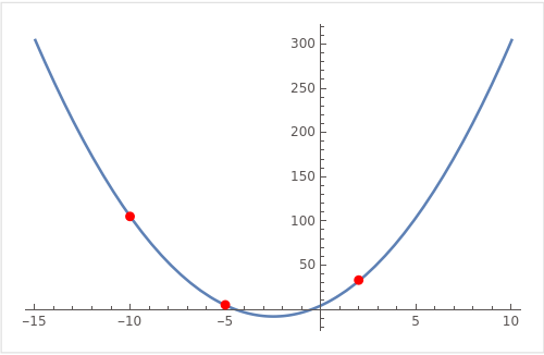
Just as two points lock down a line, three distinct points uniquely determine a quadratic polynomial (y = ax^2 + bx + c):
In 2023 Day 21 — Step Counter (2023 Notebook), Part 2 asks how many garden plots an elf can reach after (26{,}501{,}365) steps on an infinite tiling of square grids. Crucially, the target step count has the exact form (s_{\text{half}} + k \cdot W), where (s_{\text{half}}) reaches the first tile boundary and (W) is the square grid width. Because area grows quadratically as the diamond wavefront expands across identical tiles, sampling just three equidistant checkpoints (k = 0, 1, 2) gives you ((p_0, p_1, p_2)) and lets you jump straight to (k = 202{,}300) in (O(1)) time.
At (k = 0, 1, 2), Newton forward differences handle any integer-valued quadratic clean as a whistle:
\[\Delta_1 = p(1) - p(0), \qquad \Delta_2 = p(2) - 2p(1) + p(0), \qquad p(k) = p(0) + k\Delta_1 + \frac{k(k - 1)}{2}\Delta_2\]Because (k(k - 1)) is always even, integer division by 2 works exact even when the quadratic coefficient is a half-integer (such as the triangular numbers (\frac{k(k+1)}{2}), where (\Delta_2 = 1) is odd). For arbitrary non-uniform (x)-coordinates (like the (-10, 105), (-5, 5), (2, 33) curve above), fractions.Fraction Newton divided differences recover exact rational coefficients without NumPy Vandermonde float rounding:
from collections.abc import Sequence
from fractions import Fraction


def extrapolate_quadratic_012(p0: int, p1: int, p2: int, target_k: int) -> int:
    """Extrapolate integer-valued quadratic ``p(k)`` from values at ``k = 0, 1, 2``."""
    d1 = p1 - p0
    d2 = p2 - 2 * p1 + p0
    return p0 + target_k * d1 + (target_k * (target_k - 1) // 2) * d2


def fit_quadratic_exact(points: Sequence[tuple[int, int]]) -> tuple[Fraction, Fraction, Fraction]:
    """Fit exact rational coefficients ``(a, b, c)`` for ``a*x^2 + b*x + c`` from three points."""
    if len(points) != 3:
        raise ValueError("Exactly three points are required")
    (x0, y0), (x1, y1), (x2, y2) = points
    if len({x0, x1, x2}) != 3:
        raise ValueError("Three distinct x-coordinates are required")
    # Newton divided differences in exact Fraction arithmetic — zero float drift
    d01 = Fraction(y1 - y0, x1 - x0)
    d12 = Fraction(y2 - y1, x2 - x1)
    a = (d12 - d01) / (x2 - x0)
    b = d01 - a * (x0 + x1)
    c = Fraction(y0) - a * x0 * x0 - b * x0
    return a, b, c


# Equidistant sequence p(k) = 10k^2 + 20k + 10 evaluated at k = 5
assert extrapolate_quadratic_012(10, 40, 90, 5) == 360

# Odd second difference (Delta_2 = 1): triangular numbers k*(k+1)//2 at k = 5 -> 15
assert extrapolate_quadratic_012(0, 1, 3, 5) == 15

# Matches the plotted curve 2x^2 + 10x + 5 across arbitrary points
assert fit_quadratic_exact([(-10, 105), (-5, 5), (2, 33)]) == (
    Fraction(2),
    Fraction(10),
    Fraction(5),
)
Using np.polyfit(xs, ys, 2) is fine for rough plotting, yet when an AoC answer is a 15-digit integer, a single 1e-1 rounding wobble from floating-point matrix inversion will cost you a star. Stick to exact integers or Fraction.
Mixed-Integer Linear Programming with scipy.optimize.milp
When a puzzle turns linear algebra into a true optimisation problem — finding the minimum non-negative integer vector satisfying equality constraints — SymPy hits a wall.
Look at 2025 Day 10 — Factory (d10.py). Part 1 works in (\text{GF}(2)) where each button toggles lights and pressing a button twice cancels out, so BFS or small state bitmasks fly. Part 2 flips the rules: each button increments integer joltage counters by 1, targets reach hundreds, and you want the minimum total button presses:
On real inputs you routinely have 13 buttons and 10 counters. Because there are more variables than equations, the system is underdetermined. Handing (A\mathbf{x} = \mathbf{b}) to sympy.solve() yields expressions with three free parameters (x10, x11, x12), leaving you to search parameter bounds manually whilst enforcing non-negativity and integrality.
And why can’t you simply use a continuous linear program (scipy.optimize.linprog) and round the answer? Because the continuous optimum frequently sits on a fractional vertex that does not round cleanly to the nearest valid integer lattice point:
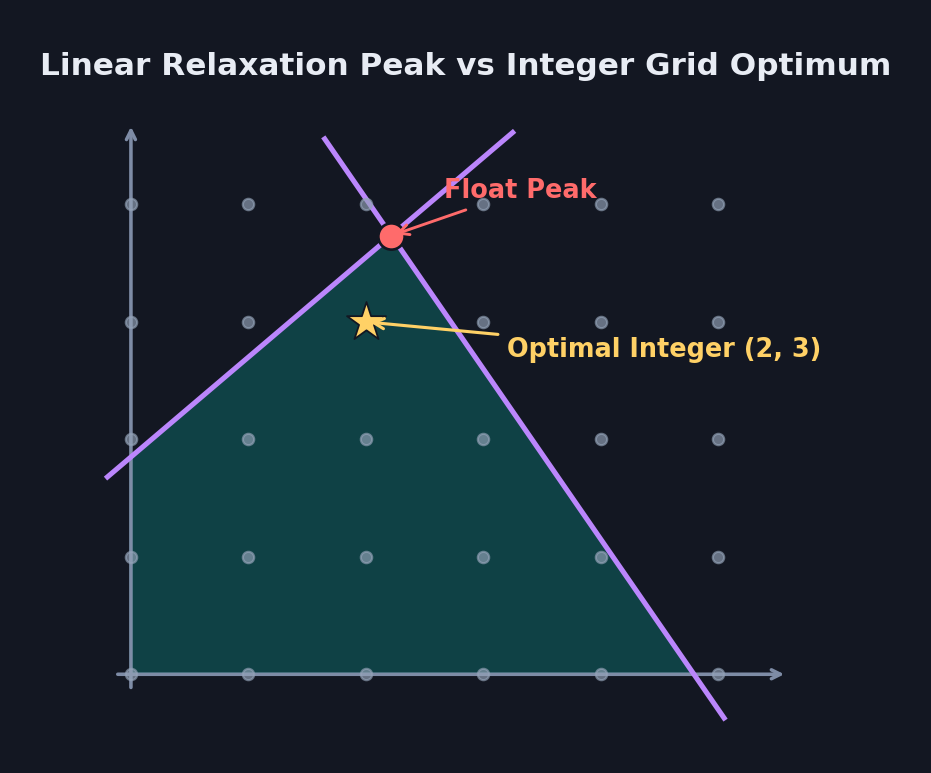
This is exactly what Mixed-Integer Linear Programming (MILP) solves out of the box via scipy.optimize.milp (backed by the HiGHS solver):
c: Cost vector per variable (np.ones(num_buttons)to minimise total presses; or[3, 1]if buttons have unequal token costs).integrality: Array of1s (np.ones(num_buttons, dtype=int)) constraining every variable to integers.bounds:Bounds(lb=0, ub=np.inf)enforcing non-negative presses.constraints:LinearConstraint(matrix_a, target, target)encoding exact equality (A\mathbf{x} = \mathbf{b}) (matching lower and upper bounds).
Two guardrails matter in practice:
- Always check
result.success(andresult.x is not None) before reading the solution. - Round carefully with
np.rint()and verify: Even integer variables come back as IEEE 754float64(e.g.2.9999999999999996), soint(val)would truncate2.9999999999999996down to2! Round withnp.rint(result.x).astype(int)and verifynp.array_equal(matrix_a @ presses, target):
import numpy as np
from scipy.optimize import Bounds, LinearConstraint, milp


def min_button_presses(
    num_counters: int,
    buttons: list[tuple[int, ...]],
    target_joltages: list[int],
) -> int:
    """Find the minimum non-negative integer button presses to match target joltages."""
    num_buttons = len(buttons)
    matrix_a = np.zeros((num_counters, num_buttons), dtype=int)
    for col, indices in enumerate(buttons):
        for row in indices:
            matrix_a[row, col] = 1

    target = np.array(target_joltages, dtype=int)
    result = milp(
        c=np.ones(num_buttons, dtype=float),
        integrality=np.ones(num_buttons, dtype=int),
        bounds=Bounds(lb=0, ub=np.inf),
        # scipy lacks bundled type stubs, so Pyright infers scalar float bounds from defaults
        constraints=LinearConstraint(matrix_a, target, target),  # pyright: ignore[reportArgumentType]
    )
    if not result.success or result.x is None:
        raise ValueError(f"No integer solution for target {target_joltages}: {result.message}")

    presses = np.rint(result.x).astype(int)
    if not np.array_equal(matrix_a @ presses, target):
        raise ValueError("Rounded MILP vector failed exact integer verification")
    return int(np.sum(presses))


# Three sample machines from 2025 Day 10
day10_samples = [
    (4, [(3,), (1, 3), (2,), (2, 3), (0, 2), (0, 1)], [3, 5, 4, 7]),
    (5, [(0, 2, 3, 4), (2, 3), (0, 4), (0, 1, 2), (1, 2, 3, 4)], [7, 5, 12, 7, 2]),
    (6, [(0, 1, 2, 3, 4), (0, 3, 4), (0, 1, 2, 4, 5), (1, 2)], [10, 11, 11, 5, 10, 5]),
]

press_counts = [min_button_presses(n, btns, tgt) for n, btns, tgt in day10_samples]
assert press_counts == [10, 12, 11]
assert sum(press_counts) == 33
Notice how concise that is — 15 lines of Python replace a custom branch-and-bound search, and every sample machine from 2025 Day 10 solves cleanly ([10, 12, 11], total 33).
1D Convex Optimisation: minimize_scalar vs Median and Mean
Sometimes the search space has only one integer variable — pick a target position (p) across a set of coordinates (x_1, \dots, x_n) to minimise total cost.
Take 2021 Day 7 — The Treachery of Whales:
-
Part 1 uses linear fuel cost (f_1(p) = \sum_{i=1}^n x_i - p ). That is an (L_1) norm sum, and its global minimum is always the median of the positions (not the mean!). -
Part 2 switches to triangular numbers (f_2(p) = \sum_{i=1}^n \frac{d_i(d_i + 1)}{2}) where (d_i = x_i - p ). Expanding (\frac{1}{2}(x_i - p)^2 + \frac{1}{2} x_i - p ) shows it is a sum of a squared error term (minimised at the mean (\mu)) plus a smaller linear term bounded by (\frac{1}{2}). Differentiating proves the continuous minimum always sits within (0.5) of the sample mean!
When you recognise that analytical shortcut, checking floor(mean) and ceil(mean) solves Part 2 in (O(n)) time. When you don’t spot the calculus trick — or when the 1D cost function is nonlinear, piecewise, or awkward to differentiate — scipy.optimize.minimize_scalar(..., method="bounded") still finds the continuous valley cleanly via Brent’s method + golden-section search.
The catch with both approaches is identical: never round a continuous minimum with round(). Because the discrete objective is asymmetric around a fractional minimum, always evaluate both math.floor(x_opt) and math.ceil(x_opt) and take the smaller integer cost:
import math
from typing import Any

import numpy as np
from scipy.optimize import minimize_scalar


def min_linear_fuel(positions: np.ndarray) -> int:
    """Minimise L1 distance sum using the exact integer median."""
    target = int(np.rint(np.median(positions)))
    return int(np.sum(np.abs(positions - target)))


def min_triangular_fuel_scipy(positions: np.ndarray) -> int:
    """Minimise triangular fuel cost via 1D convex search checked at adjacent integers."""

    def cost(pos: float) -> float:
        dist = np.abs(positions - pos)
        return float(np.sum(dist * (dist + 1) / 2))

    res: Any = minimize_scalar(
        cost,
        bounds=(float(positions.min()), float(positions.max())),
        method="bounded",
    )
    # Check both floor and ceil because rounding a continuous valley can pick the wrong side
    candidates = {math.floor(float(res.x)), math.ceil(float(res.x))}
    return min(
        int(np.sum((d := np.abs(positions - p)) * (d + 1) // 2))
        for p in candidates
    )


def min_triangular_fuel_mean(positions: np.ndarray) -> int:
    """Minimise triangular fuel cost analytically within 0.5 of the sample mean."""
    mean = float(np.mean(positions))
    candidates = {math.floor(mean), math.ceil(mean)}
    return min(
        int(np.sum((d := np.abs(positions - p)) * (d + 1) // 2))
        for p in candidates
    )


crabs = np.array([16, 1, 2, 0, 4, 2, 7, 1, 2, 14], dtype=int)
assert min_linear_fuel(crabs) == 37
assert min_triangular_fuel_scipy(crabs) == 168
assert min_triangular_fuel_mean(crabs) == 168
On the sample [16, 1, 2, 0, 4, 2, 7, 1, 2, 14], the mean is 4.9: position 4 costs 170 fuel whilst position 5 costs 168. On full inputs, the opposite frequently happens (x.5 leaning towards floor), which is why checking {math.floor(...), math.ceil(...)} is cheap insurance. See NumPy for more array broadcasting helpers.
Constraint Propagation and Stack Deduction
Bipartite Singleton Peeling
A surprising fraction of AoC logic puzzles are disguised bipartite 1-to-1 matching problems:
- 2020 Day 16 — Ticket Translation (
ticket_processor.py): match each ticket column index to a valid field rule. - 2020 Day 21 — Allergen Assessment (
ingredients.py): match each allergen to the single ingredient present in every food listing it. - 2021 Day 8 — Seven Segment Search: deduce scrambled digit and segment mappings by intersecting and subtracting candidate sets.
In every one of these puzzles, intersecting candidate sets (Sets + Defaultdict) narrows each unknown down until at least one key has exactly one candidate remaining. Assigning that forced singleton removes its value from every other candidate set, revealing the next singleton in a cascade.
Rather than rewriting that while loop each December, extract a generic PEP 695 helper — failing loudly if a contradiction or ambiguity leaves no singletons to peel:
from collections.abc import Iterable, Mapping


def resolve_unique_assignments[K, V](candidates: Mapping[K, Iterable[V]]) -> dict[K, V]:
    """Resolve a 1-to-1 assignment by iteratively peeling forced singletons."""
    remaining: dict[K, set[V]] = {key: set(values) for key, values in candidates.items()}
    resolved: dict[K, V] = {}

    while remaining:
        singletons = [(key, next(iter(opts))) for key, opts in remaining.items() if len(opts) == 1]
        if not singletons:
            raise ValueError(f"Constraint system is underconstrained or inconsistent: {remaining}")

        for key, value in singletons:
            if value in resolved.values():
                raise ValueError(f"Duplicate forced assignment for value {value!r}")
            resolved[key] = value
            del remaining[key]

        assigned_values = {value for _, value in singletons}
        for opts in remaining.values():
            opts.difference_update(assigned_values)
            if not opts:
                raise ValueError("Candidate set became empty during constraint propagation")

    return resolved


# Sample allergen candidates after intersecting food lists (2020 Day 21)
allergen_candidates = {
    "dairy": {"mxmxvkd"},
    "fish": {"mxmxvkd", "sqjhc"},
    "soy": {"sqjhc", "fvjkl"},
}
assert resolve_unique_assignments(allergen_candidates) == {
    "dairy": "mxmxvkd",
    "fish": "sqjhc",
    "soy": "fvjkl",
}
Paired Push/Pop Stack Constraints
Every few years, an AoC assembly or VM puzzle looks intractable — (9^{14}) valid 14-digit model numbers in 2021 Day 24 — Arithmetic Logic Unit — until you print the instruction blocks side by side and discover they aren’t arbitrary at all.
In Day 24, the ALU uses register z as a base-26 stack:
- Seven blocks divide
zby1(div z 1) and always fail the branch check, unconditionally pushingdigit[i] + add_yontoz. - Seven matching blocks divide
zby26(div z 26), popping the top entry and requiringdigit[j] == popped + check_xin order to finish withz == 0.
Once you pair each push block (push_idx, add_y) with its matching pop block (pop_idx, check_x) using a plain list stack, every pair yields a tiny linear difference constraint:
To maximise the 14-digit string, push digit[i] as high as 9 allows (min(9, 9 - delta)); to minimise it, push digit[i] as low as 1 allows (max(1, 1 - delta)). Seven stack pops solve a (2.28 \times 10^{13}) search space in microseconds:
def solve_paired_stack_bounds(
    block_params: list[tuple[int, int, int]],
    *,
    maximise: bool = True,
) -> str:
    """Solve base-26 push/pop digit constraints in linear time using a stack."""
    digits = [0] * len(block_params)
    stack: list[tuple[int, int]] = []  # (push_index, push_offset)

    for idx, (div_z, check_x, add_y) in enumerate(block_params):
        if div_z == 1:
            stack.append((idx, add_y))
            continue
        if div_z != 26:
            raise ValueError(f"Expected div_z in 1, got {div_z}")
        if not stack:
            raise ValueError(f"Unmatched pop block at index {idx}")

        push_idx, push_offset = stack.pop()
        delta = push_offset + check_x  # digit[idx] - digit[push_idx] == delta
        push_digit = min(9, 9 - delta) if maximise else max(1, 1 - delta)
        pop_digit = push_digit + delta
        if not (1 <= push_digit <= 9 and 1 <= pop_digit <= 9):
            raise ValueError(f"No valid digits 1..9 for delta={delta}")
        digits[push_idx] = push_digit
        digits[idx] = pop_digit

    if stack:
        raise ValueError("Unmatched push blocks remain on stack")
    return "".join(str(d) for d in digits)


# Synthetic 4-block trace: d2 == d1 + 2 and d3 == d0 + 3
synthetic_alu = [
    (1, 12, 4),   # push d0 + 4
    (1, 11, 7),   # push d1 + 7
    (26, -5, 2),  # pop -> d2 == d1 + (7 - 5) == d1 + 2
    (26, -1, 1),  # pop -> d3 == d0 + (4 - 1) == d0 + 3
]
assert solve_paired_stack_bounds(synthetic_alu, maximise=True) == "6799"
assert solve_paired_stack_bounds(synthetic_alu, maximise=False) == "1134"
AoC Examples
| Puzzle | Mathematical / Constraint Pattern | Solution Link |
|---|---|---|
| 2020 Day 16 — Ticket Translation | Bipartite singleton peeling over valid field-to-column sets | ticket_processor.py (2020 Hub) |
| 2020 Day 21 — Allergen Assessment | Set intersection followed by resolve_unique_assignments |
ingredients.py (2020 Hub) |
| 2021 Day 7 — The Treachery of Whales | Median ((L_1)) vs minimize_scalar / mean (\pm 0.5) checked at floor/ceil |
2021 Day 7 |
| 2021 Day 8 — Seven Segment Search | Set-algebra candidate elimination (plus 7! permutation search) |
2021 Day 8 |
| 2021 Day 24 — Arithmetic Logic Unit | Base-26 stack push/pop paired digit constraints | 2021 Day 24 |
| 2023 Day 21 — Step Counter | 3-point equidistant quadratic finite differences | 2023 Notebook (2023 Hub) |
| 2024 Day 13 — Claw Contraption | Exact integer (2 \times 2) Cramer’s rule via divmod at (10^{13}) scale |
2024 Notebook (2024 Hub) |
| 2025 Day 10 — Factory | Underdetermined non-negative integer minimisation via scipy.optimize.milp |
2025 Day 10 (d10.py) |