Learning Python with Advent of Code Walkthroughs
Dazbo's Advent of Code solutions, written in Python
The Python Journey - Maths with SymPy

Useful Links
Page Contents
Work in progress…
What is SymPy?
SymPy is so cool! I came across when I was trying to solve some equations as part of 2023 AoC puzzles. It is computer alegebra systems (CAS): a library that allows us to perfrom algebra and mathematical computations.
You can use it for things like:
- Simplifying, rearranging, factoring and expanding algebraic expressions and equations.
- Solving equations of various types, including linear, polynomial, and differential.
- Performing calculus, including differentiation and integration.
- Plotting graphs.
- Generating LaTeX output.
Basic Examples
Simplifying and Expanding
We need to define variables before we can use them in SymPy. We do this by creating symbols.
One interesting observation here is that when you evaluate a SymPy expression a Jupyter notebook, it is rendered in pretty-printed (mathematical) format. But when we print using print(), it is printed in conventional Python style.
If you want to explicitly pretty-print from a Python notebook, you can use IPython.display.
Alternatively, you can optionally run init_printing() to enable the best printer for your environment. Or run init_session() to automatically import everything in SymPy, create some common Symbols, setup plotting, and run init_printing().
import sympy
from sympy import latex
from IPython.display import display, Markdown
sympy.init_session() # set up default behavour and printing - not essential
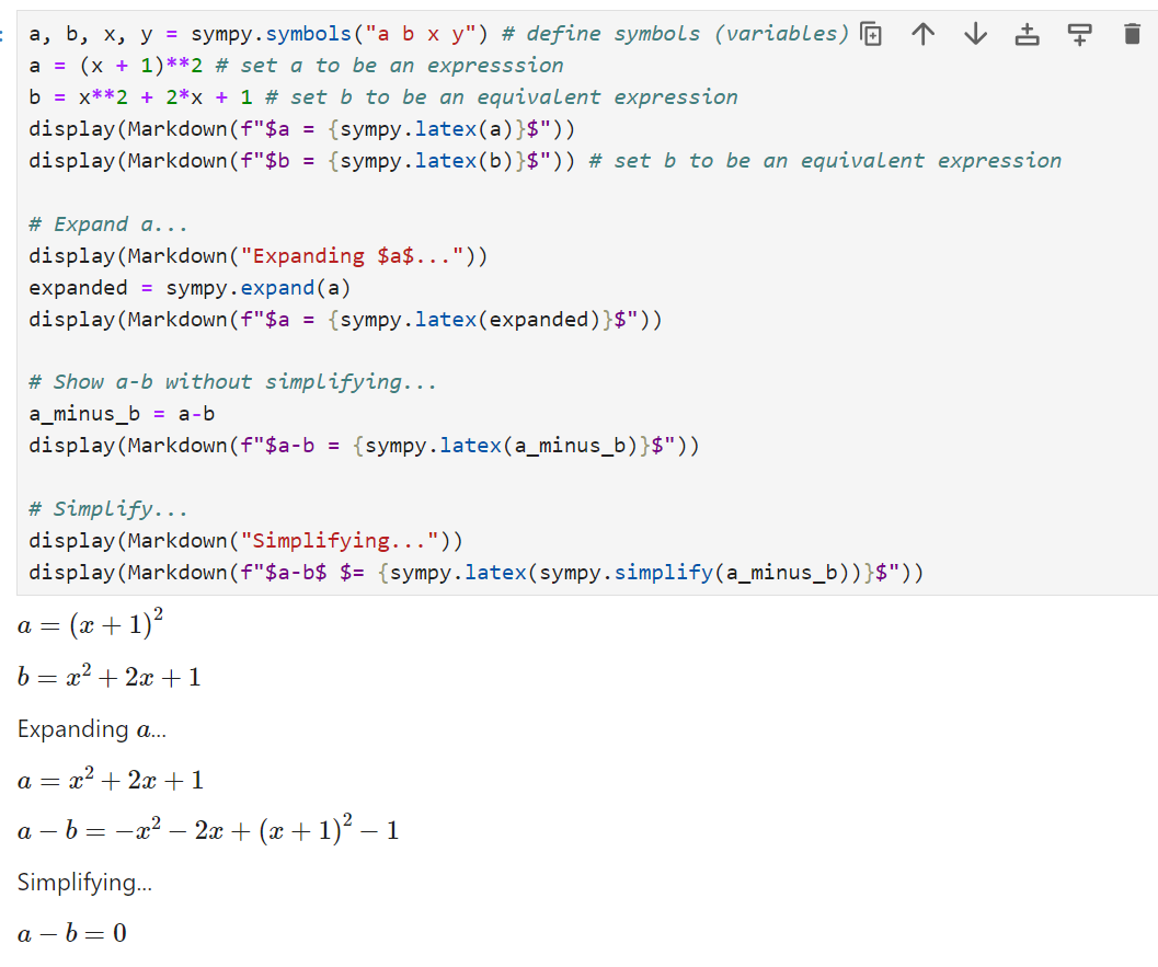
a, b, x, y = sympy.symbols("a b x y") # define symbols (variables)
a = (x + 1)**2 # set a to be an expresssion
b = x**2 + 2*x + 1 # set b to be an equivalent expression
display(Markdown(f"$a = {latex(a)}$")) # pretty-print a
print(f"{latex('a = ')}{latex(a)}") # If we just want the raw latex
display(Markdown(f"$b = {latex(b)}$")) # pretty-print b
# Expand a...
display(Markdown("Expanding $a$..."))
expanded = sympy.expand(a)
display(Markdown(f"$a = {latex(expanded)}$"))
# Show a-b without simplifying...
a_minus_b = a-b
display(Markdown(f"$a-b = {latex(a_minus_b)}$"))
# Simplify...
display(Markdown("Simplifying..."))
display(Markdown(f"$a-b$ $= {latex(sympy.simplify(a_minus_b))}$"))
We can also test if two expressions are the same, e.g.
a.equals(b)
Assigning Variables and Evaluating
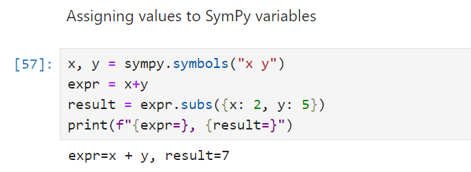
You can’t simply assign values to the Python variable. If you did so, they would cease to be a symbol. Instead, you need to use subs() to associate a value with a SymPy symbol.
x, y = sympy.symbols("x y")
expr = x+y
result = expr.subs({x: 2, y: 5})
print(f"{expr=}, {result=}")
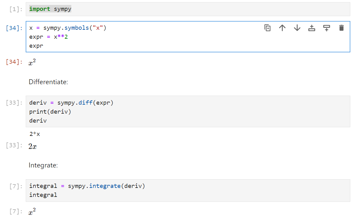
Differentiation and Integration
import sympy

x = sympy.symbols("x")
expr = x**2

deriv = sympy.diff(expr)
print(deriv)

integral = sympy.integrate(deriv)
print(integral)
Solving Quadratics
Here, I use solve() to determine the values of $x$. I’ve specified dict=True such that $x$ can be retrieved by passing its symbol as a dictionary key to the returned solutions dictionary.
expr = x**2 + 3*x - 10
solutions = sympy.solve(expr, x, dict=True)
solutions

for solution in solutions:
    print(f"x={solution[x]}")
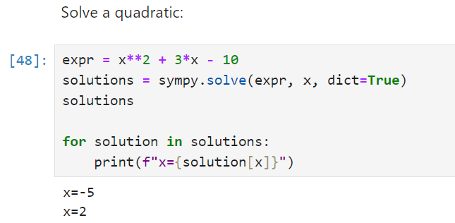
Note that the expressions still need to be written in valid Python. So we can write 3*x, but we can’t write 3x.
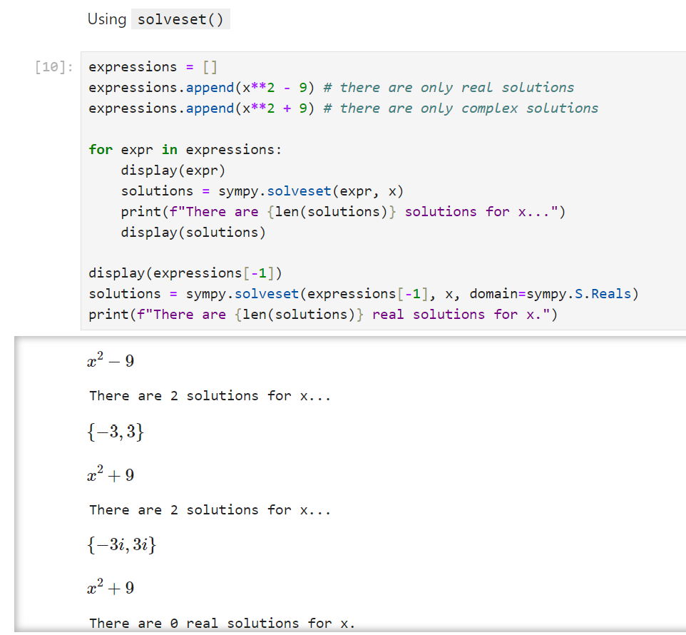
Including Only Real Solutions
What if you want to ignore complex solutions and only include real solutions? In this case, you can use solveset(), and specify the domain as domain=sympy.S.Reals. (Whereas domain=S.Complexes is the default.)
expressions = []
expressions.append(x**2 - 9) # there are only real solutions
expressions.append(x**2 + 9) # there are only complex solutions

for expr in expressions:
    display(expr)
    solutions = sympy.solveset(expr, x)
    print(f"There are {len(solutions)} solutions for x...")
    display(solutions)

display(expressions[-1])
solutions = sympy.solveset(expressions[-1], x, domain=sympy.S.Reals)
print(f"There are {len(solutions)} real solutions for x.")
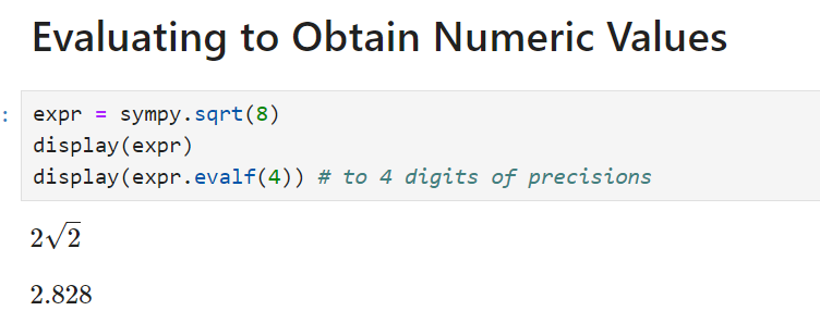
Evaluating to Obtain Numeric Values
We can evaluate to obtain the float value of a symbol, and display to an arbitrary level of precision:
expr = sympy.sqrt(8)
display(expr)
display(expr.evalf(4)) # to 4 digits of precisions
AoC Examples
Boat Racing Quadratic
In this example taken from 2023 Day 6, I’m solving a quadratic:
\[h^2 - th + d = 0\]def solve_part2_sympy_quadratic(data):
""" h^2 - th + d = 0 """
race_duration = int("".join(x for x in data[0].split(":")[1].split()))
distance = int("".join(x for x in data[1].split(":")[1].split()))
logger.debug(f"{race_duration=}, {distance=}")
# solve using quadratic with SymPy
h = sympy.symbols("h", real=True)
equation = sympy.Eq(h**2 - race_duration*h + distance, 0)
solutions = sympy.solve(equation, h, dict=True)
answers = [solution[h].evalf() for solution in solutions] # there should be two
Trajectory Intersection
In this example taken from 2023 Day 24, I have a series of equations that are necessary to find several unknown variables. Specifically:
\[\begin{align} t &= \frac{x_{r} - x_{h}}{v_{x_{h}} - v_{x_{r}}} = \frac{y_{r} - y_{h}}{v_{y_{h}} - v_{y_{r}}} = \frac{z_{r} - z_{h}}{v_{z_{h}} - v_{z_{r}}} \\ \notag \\ (x_{r} - x_{h})(v_{y_{h}} - v_{y_{r}}) &= (y_{r} - y_{h})(v_{x_{h}} - v_{x_{r}}) \\ (y_{r} - y_{h})(v_{z_{h}} - v_{z_{r}}) &= (z_{r} - z_{h})(v_{y_{h}} - v_{y_{r}}) \\ (z_{r} - z_{h})(v_{x_{h}} - v_{x_{r}}) &= (x_{r} - x_{h})(v_{z_{h}} - v_{z_{r}}) \\ \end{align}\]And here’s the code:
def solve_part2(data: list[str]):
    """
    Determine the sum of the rock's (x,y,z) coordinate at t=0, for a rock that will hit every hailstone
    in our input data. The rock has constant velocity and is not affected by collisions.
    """
    stones = parse_stones(data)
    logger.debug(f"We have {len(stones)} stones.")

    # define SymPy rock symbols - these are our unknowns representing:
    # initial rock location (xr, yr, zr)
    # rock velocity (vxr, vyr, vzr)
    xr, yr, zr, vxr, vyr, vzr = sympy.symbols("xr yr zr vxr vyr vzr")

    equations = [] # we assemble a set of equations that must be true
    for stone in stones[:10]: # we don't need ALL the stones to find a solution. We need just enough.
        x, y, z = stone.posn
        vx, vy, vz = stone.velocity
        equations.append(sympy.Eq((xr-x)*(vy-vyr), (yr-y)*(vx-vxr)))
        equations.append(sympy.Eq((yr-y)*(vz-vzr), (zr-z)*(vy-vyr)))

    solutions = sympy.solve(equations, dict=True) # SymPy does the hard work
    if solutions:
        solution = solutions[0]
        logger.info(solution)
        return sum([solution[xr], solution[yr], solution[zr]])

    logger.info("No solutions found.")
    return None