Learning Python with Advent of Code Walkthroughs
Dazbo's Advent of Code solutions, written in Python
The Python Journey - Creating and Visualising Graphs with NetworkX
Useful Links
Graphs and Graph TheoryNetworkXCustomising NetworkX GraphsMatplotlib
Page Contents
- Introduction
- Installing NetworkX
- NetworkX Guides and Tutorials
- Getting Started With NetworkX
- Supplying Graph Data
- Drawing the Graph
- More Interesting Graphs
- Examples
Introduction
NetworkX is a cool library that allows us to create, manipulate, interrogate, and render graphs. It can take a lot of the pain out of building graphs. It also has cool methods that allow us to do things like: find the shortest path from a to b. And it can also render the graph as an image for us.
Installing NetworkX
py -m pip install networks
NetworkX Guides and Tutorials
Here are a few useful links:
- NetworkX Tutorial
- NetworkX Reference
- Examples Gallery
- Layouts
- Algorithms
- Customizing NetworkX Graphs
Getting Started With NetworkX
We need to import the relevant packages. You’ll probably want to import matplotlib.pyplot if you want to render any graph visualisations.
import networkx as nx
import matplotlib.pyplot as plt
Supplying Graph Data
Typically, we’ll want to build a graph by supplying edge information. I.e. a connection between one node and another.
For example, let’s say we have a list of input data, where each line of data contains two locations. We might build an unweighted, undirected graph like this:
def build_graph(data) -> nx.Graph:
    """ Build graph from list of connected points.

    Args:
        data (list[str]): pairs of points, in the form "Name_X connected to Name_Y"

    Returns:
        dict: (start, end) = distance
    """
    graph = nx.Graph()
    points_match = re.compile(r"^(\w+) connected to (\w+)")

    # Add each edge, in the form of a location pair
    for edge in data:
        start, end = points_match.findall(edge)[0]
        graph.add_edge(start, end)

    return graph
Or, if we also have some sort of weight information (e.g. distance between points, cost of a route, etc), then we can build a directed graph like this:
def build_graph(data) -> nx.Graph:
    """ Build graph from list of connected points.

    Args:
        data (list[str]): pairs of points, in the form "Name_X to Name_Y = distance_n"

    Returns:
        dict: (start, end) = distance
    """
    graph = nx.Graph()
    distance_match = re.compile(r"^(\w+) to (\w+) = (\d+)")

    # Add each edge, in the form of a location pair
    for edge in data:
        start, end, distance = distance_match.findall(edge)[0]
        distance = int(distance)
        graph.add_edge(start, end, distance=distance)

    return graph
Or we could be a directed weighted graph, like this:
def build_graph(rules):
    """ Builds a graph from a dict of rules

    Args:
        rules (dict): Look like... 'shiny plum': {'dotted beige': 5, 'faded orange': 1}

    Returns:
        nx.DiGraph: Directed graph
    """
    graph = nx.DiGraph()
    for parent, children in rules.items():
        graph.add_node(parent)
        for child, child_count in children.items():
            graph.add_node(child)
            graph.add_edge(parent, child, count=child_count)
    return graph
We can also create our edges from various data structures, such as from a Pandas DataFrame, using nx.from_pandas_edgelist().
Drawing the Graph
Having built a graph, we can then render it as a visualisation.
The basic functon is draw().
E.g.
nx.draw(graph, with_labels=True, node_color='blue')
Note that NetworkX must decide where to position each node on the drawing canvas. This is done by supplying a layout to NetworkX. If you don’t supply one, NetworkX uses ‘spiral’ by default.
There are two ways you can supply a layout.
- You can supply a layout and obtain on the positions. You then use these positions in later calls.
- You can use the
draw_xxx()method, wherexxxis one of the supported layouts.
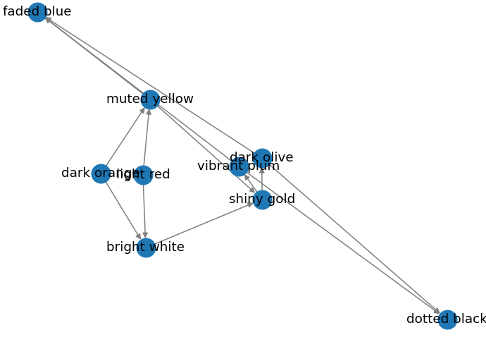
In the following examples, I’ll render directed, weighted output with the following data, and using a number of different layouts.
light red bags contain 1 bright white bag, 2 muted yellow bags.
dark orange bags contain 3 bright white bags, 4 muted yellow bags.
bright white bags contain 1 shiny gold bag.
muted yellow bags contain 2 shiny gold bags, 9 faded blue bags.
shiny gold bags contain 1 dark olive bag, 2 vibrant plum bags.
dark olive bags contain 3 faded blue bags, 4 dotted black bags.
vibrant plum bags contain 5 faded blue bags, 6 dotted black bags.
faded blue bags contain no other bags.
dotted black bags contain no other bags.
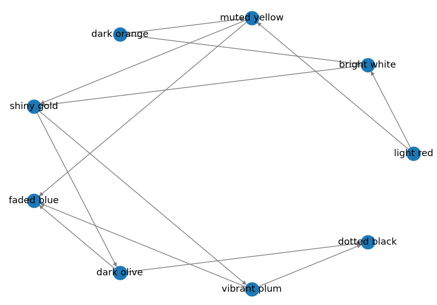
Spring Layout (Default)
def draw_graph(graph):
    nx.draw(graph, edge_color="grey", width=1, with_labels=True)
    ax = plt.gca()
    ax.set_axis_off()
    plt.show()
Or equivalent:
def draw_graph(graph, searching_for, ancestors):
    pos = nx.spring_layout(graph)
    nx.draw(graph, pos=pos, edge_color="grey", width=1, with_labels=True)
    ax = plt.gca()
    ax.set_axis_off()
    plt.show()
Output:
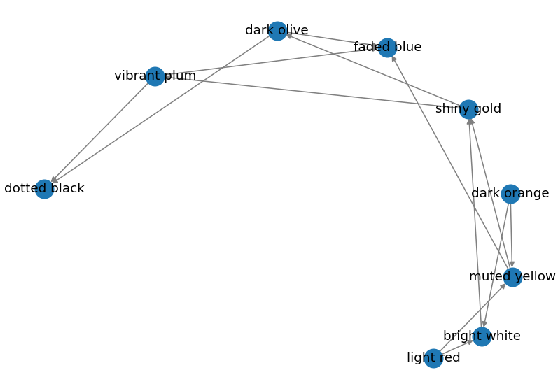
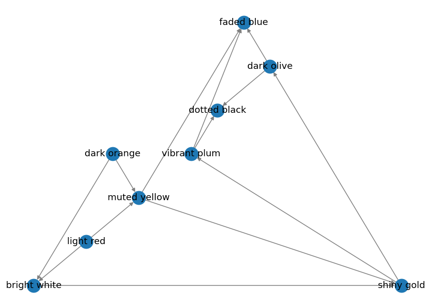
Spiral Layout
pos = nx.spiral_layout(graph)
nx.draw(graph, pos=pos, edge_color="grey", width=1, with_labels=True)
Output:
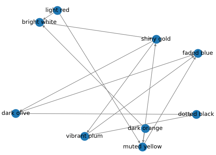
Circular Layout
pos = nx.circular_layout(graph)
nx.draw(graph, pos=pos, edge_color="grey", width=1, with_labels=True)
Output:
Planar Layout
pos = nx.planar_layout(graph)
nx.draw(graph, pos=pos, edge_color="grey", width=1, with_labels=True)
Output:
Random Layout
pos = nx.random_layout(graph)
nx.draw(graph, pos=pos, edge_color="grey", width=1, with_labels=True)
Output:
More Interesting Graphs
The graphs above are quite boring. So let’s look at how we can make them more interesting and valuable.
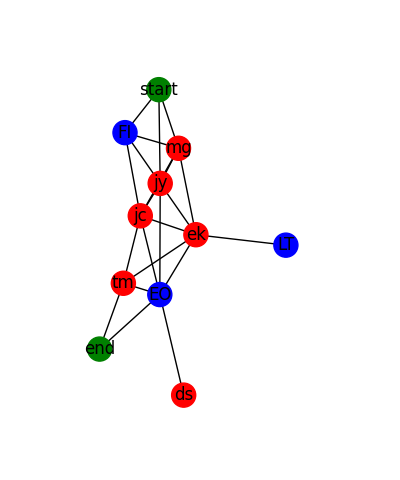
Colouring Nodes Based on Attributes
Here we examine each node in the supplied graph, and then colour the nodes based on specific attributes.
- The the node is one of START or END, we colour it in green.
- If the node is one of a list of nodes called
special_nodes, then we colour it blue. - Otherwise, we colour it red.
This works by creating a list of colours, which has the same number of elements as graph.nodes, and is in the same order as the nodes. We must pass this list to our draw() method.
def render(graph, START, END, special_nodes, file):
    _ = plt.subplot(121)  # throwaway variable
    pos = nx.spring_layout(self._graph)

    # set colours for each node in the array, in the same order as the nodes
    colours = []
    for node in graph.nodes:
        if node in (START, END):
            colours.append("green")
        elif node in special_nodes:
            colours.append("blue")
        else:
            colours.append("red")

    nx.draw(graph, pos=pos, node_color=colours, with_labels=True)

    dir_path = Path(file).parent
    if not Path.exists(dir_path): # Create output folder if it doesn't exist
        Path.mkdir(dir_path)
    plt.savefig(file)   # save the visualisation as a file
The output looks like this:
Colouring a Particular Path
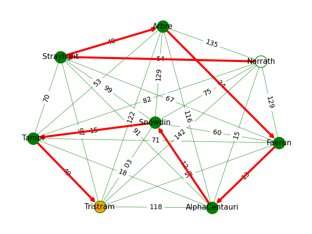
In the example below, we:
- Draw a weighted graph that shows a number of locations as nodes, and a number of edges as distances between nodes.
- We also superimpose a specific route that we want to highlight.
To achieve this, we:
- Draw all the nodes in green, except the start and end nodes of our route. (Note that the locations in the
routemust be nodes from the graph itself.) - Label all the nodes.
- Add the start and end nodes from our route, colouring them white and orange, respectively.
- Draw all the edges, with a thin green line.
- Add the edge labels, i.e. the distances of each edge. (Remember that this is a weighted graph, and the weight of each edge is the distance.)
- Finally, we redraw all the edges from our route, with direction, with heavy red lines. We use the convenience method
nx.utils.pairwise(route)to obtain the edges between each adjacent node in the suppliedroute.
def draw_graph(graph, route):
    start_node = route[0]
    end_node = route[-1]

    pos = nx.spring_layout(graph) # create a layout for our graph

    # Draw all nodes in the graph
    nx.draw_networkx_nodes(graph, pos,
                           nodelist=route[1:-1], # exclude start and end
                           node_color="green")

    # Draw all the node labels
    nx.draw_networkx_labels(graph, pos, font_size=11)

    # Draw start and end nodes
    nx.draw_networkx_nodes(graph, pos, nodelist=[start_node],
                           node_color="white", edgecolors="green")
    nx.draw_networkx_nodes(graph, pos, nodelist=[end_node],
                           node_color="orange", edgecolors="green")

    # Draw closest edges for each node only - with thin lines
    nx.draw_networkx_edges(graph, pos,
                           edge_color="green", width=0.5)

    # Draw all the edge labels - i.e. the distances
    nx.draw_networkx_edge_labels(graph, pos, nx.get_edge_attributes(graph, DISTANCE))

    # Draw the edges that make up this particular route
    route_edges = list(nx.utils.pairwise(route))
    nx.draw_networkx_edges(graph, pos, edgelist=route_edges,
                           edge_color="red", width=3, arrows=True)

    ax = plt.gca()
    plt.axis("off")
    plt.tight_layout()
    plt.show()
The visualisation looks like this:
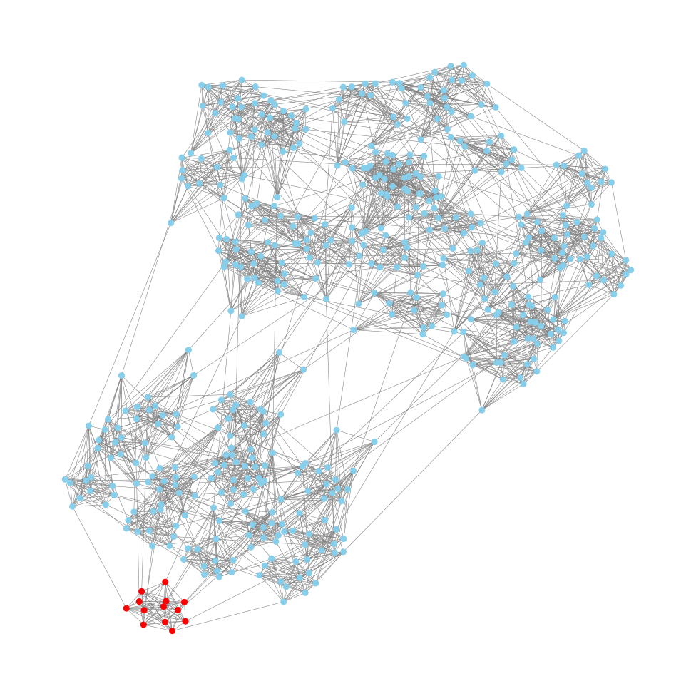
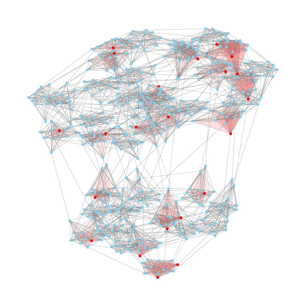
Identifying Cliques
This is taken from AoC 2024 Day 23 - LAN Party
A clique is a subset of vertices such that every two distinct vertices are adjacent. What this means is that there is an edge between every pair of nodes in the clique. To put it another way: every node in the subset is directly connected to every other node.
Let’s say we have a list of connected nodes:
kh-tc
qp-kh
de-cg
ka-co
yn-aq
qp-ub
We can identify cliques like this:
def identify_triangle_cliques(data: list[str], real=True):
    graph = nx.Graph()
    for line in data:
        if not line.strip():
            continue

        a, b = line.split("-")
        graph.add_edge(a, b)

    logger.debug(f"{len(graph)=}, {graph=}")

    # Find all triangles in the graph
    # A clique is a set of nodes where every pair is connected
    triangles = [set(triangle) for triangle in nx.enumerate_all_cliques(graph)
                               if len(triangle) == 3]

    logger.debug(f"{len(triangles)=}, {triangles=}")

    chief_candidates = [triangle for triangle in triangles
                                 if any(node.startswith("t") for node in triangle)]
    logger.debug(f"{len(chief_candidates)=}, {chief_candidates=}")

    visualise_graph(graph, real=real, chief_candidates=chief_candidates)
    return len(chief_candidates)

def visualise_graph(graph, real, chief_candidates=None, largest_clique=None):
    fig, ax = plt.subplots(figsize=(12, 12), dpi=80)

    if real:
        node_size =  50
        width = 0.5
        with_labels = False
        alpha=0.01
    else:
        node_size = 500
        width = 1
        with_labels = True
        alpha=0.1

    pos = nx.spring_layout(graph)
    if chief_candidates:
        node_color = [('red' if node.startswith("t") else 'skyblue') for node in graph]
        for triangle in chief_candidates:
            # Add semi-transparent triangles
            vertices = [pos[node] for node in triangle]
            poly = Polygon(vertices, alpha=alpha, facecolor='red', edgecolor='none')
            ax.add_patch(poly)
    else:
        assert largest_clique, "Largest clique not set"
        node_color = [('red' if node in largest_clique else 'skyblue') for node in graph]

    nx.draw(
        graph, pos=pos,
        edge_color="grey", width=width, with_labels=with_labels,
        node_color=node_color,
        node_size=node_size,
    )
    fig.tight_layout(pad=0)

    ax = plt.gca()
    ax.set_axis_off()
    plt.show()
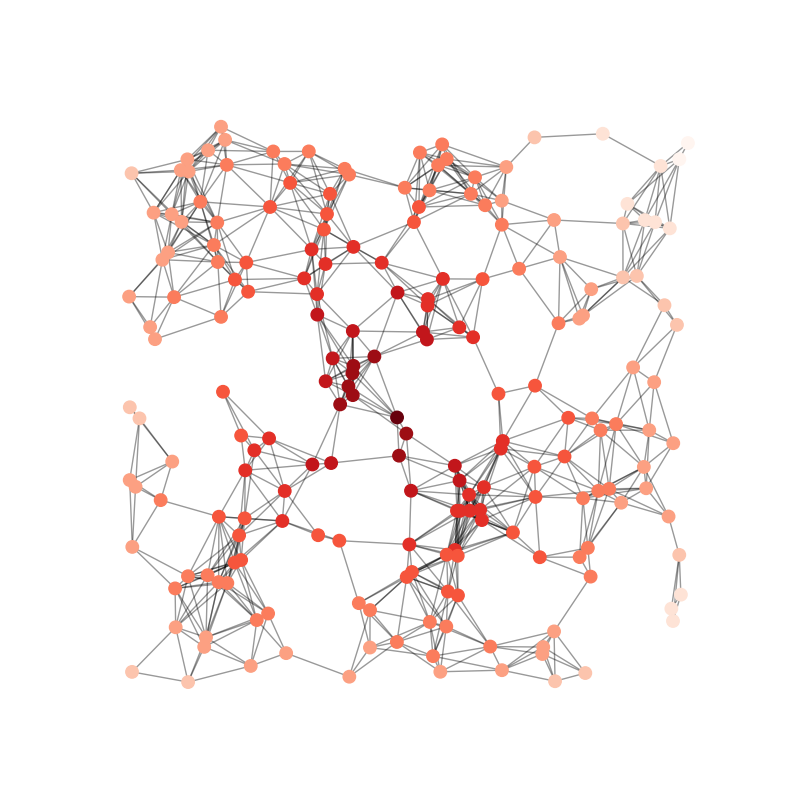
Find Maximal Cliques
This is taken from AoC 2024 Day 23 - LAN Party
A maximal clique is a clique that cannot be extended by adding more nodes while remaining fully connected. So we can just retrieve all the maximal cliques, and then return the one that is largest. I.e. the largest clique where all nodes are directly connected to each other.
def solve_part2(data, real=True):
    graph = nx.Graph()
    for line in data:
        if not line.strip():
            continue

        a, b = line.split("-")
        graph.add_edge(a, b)

    # Find maximal cliques
    maximal_cliques = list(nx.find_cliques(graph))
    largest_clique = max(maximal_cliques, key=len)

    logger.debug(f"{len(largest_clique)=}, {largest_clique=}")
    visualise_graph(graph, real=real, largest_clique=largest_clique)

    return ",".join(sorted(largest_clique))