Advent of Code 2021 - Day 15

Useful Links

Concepts and Packages Demonstrated

dataclassPriority queuevisualisation

Problem Intro

We’re in a cavern with a low ceiling just above us, so we can only navigate in two dimensions. I.e. we can’t go up or down. The cavern makes up a graph of connected locations that we need to navigate through. We’re told that the cave walls are covered in chitons, and don’t want to bump into them!

Our sub’s computer has mapped out the chiton density, and converted this into grid of risk level, in the two dimensions we can navigate.

The input data looks like this:

We start in the top left. We can navigate the maze by moving in any orthogonal direction; we can’t move diagonally.

Part 1

We need to get to the bottom right, and we need to compute the total risk of the lowest risk route. Total risk is given by adding up the risk of every location we enter; thus, the risk of our starting location is not counted.

Setup

The usual stuff…

from __future__ import annotations
from copy import deepcopy
from dataclasses import dataclass
import logging
import os
import time
import heapq

SCRIPT_DIR = os.path.dirname(__file__) 
INPUT_FILE = "input/input.txt"
# INPUT_FILE = "input/sample_input.txt"

logging.basicConfig(format="%(asctime)s.%(msecs)03d:%(levelname)s:%(name)s:\t%(message)s", 
                    datefmt='%H:%M:%S')
logger = logging.getLogger(__name__)
logger.setLevel(level=logging.DEBUG)

The only new addition worthy of mention is the heapq module. This allows us to implement a priority queue. More on this later.

Solution

This is simple enough. We’re going to use a bog-standard Dijkstra solution.

Recall that in Day 9 we used a Breadth First Search (BFS) to flood fill an area. And in Day 12 we again used the BFS to find all the paths between a starting point and a destination.

Well, Dijkstra builds on the BFS algorithm, by allowing us to prioritise the paths we want to explore first, favouring paths with a lower cost. Thus, Dijkstra is a great algorithm to allow us to find the best path through a graph, where best might mean shortest, fastest, lowest_cost, etc. It’s also particularly suited to where movement in the graph may have variable cost.

And this is exactly the scenario we have here: some locations have higher risk scores. So, we want to prioritise the path that has the overall lowest risk cost.

The Dijkstra works just like the BFS, in that it uses a frontier that expands in all valid directions. However, unlike a BFS where we typically pop items off the frontier in the order they were added (FIFO), Dijkstra instead uses a priority queue for the frontier, where we pop off items that have the lowest priority. (Here, lowest could actually be highest; it really depends what behaviour you want.)

For our solution, we want to prioritise based on lowest cumulative risk. So, we do this by keeping track of our path and the total risk for our path. And as we explore the next possible move for each path, we always explore the path that has the lowest cumulative risk, first.

We’ll start with a Point dataclass:

@dataclass(frozen=True, order=True)
class Point():
    """ Point class, which knows how to return a list of all adjacent coordinates """
    
    # Return all adjacent orthogonal (not diagonal) coordinates
    DELTAS = [(dx,dy) for dx in range(-1, 2) for dy in range(-1, 2) if abs(dy) != abs(dx)]
    
    x: int
    y: int
    
    def neighbours(self) -> list[Point]:
        """ Return all adjacent orthogonal (not diagonal) Points """
        return [Point(self.x+dx, self.y+dy) for dx,dy in Point.DELTAS]

Now let’s create a Grid class to represent our input of risks:

class Grid():
    """ 2D grid of point values. Knows how to:
       - Determine value at any point
       - Determine all neighbouring points of a given point """
       
    def __init__(self, grid_array: list[list[int]]) -> None:
        """ Generate Grid instance from 2D array. 
        This works on a deep copy of the input data, so as not to mutate the input. """                                         
        self._array = deepcopy(grid_array)  # Store a deep copy of input data
        self._x_size = len(self._array[0])
        self._y_size = len(self._array)
        
    @property
    def x_size(self):
        """ Array width (cols) """
        return self._x_size
    
    @property
    def y_size(self):
        """ Array height (rows) """
        return self._y_size
    
    @property
    def array(self):
        return self._array

    def all_points(self) -> list[Point]:
        points = [Point(x, y) for x in range(self.x_size) for y in range(self.y_size)]
        return points
    
    def set_value_at_point(self, point: Point, value: int):
        self._array[point.y][point.x] = value
        
    def value_at_point(self, point: Point) -> int:
        """ Value at this point """
        return self._array[point.y][point.x]
    
    def _valid_location(self, point: Point) -> bool:
        """ Check if a location is within the grid """
        if (0 <= point.x < self.x_size and 0 <= point.y < self.y_size):
            return True
        
        return False
    
    def valid_neighbours(self, point:Point):
        """ Yield adjacent neighbour points """
        for neighbour in point.neighbours():
            if self._valid_location(neighbour):
                yield neighbour
    
    def __repr__(self) -> str:
        return "\n".join("".join(map(str, row)) for row in self._array)

There’s not much to say about this. We’ve seen it all before.

We initialise with a deepcopy of the input, so that we can modify the data internally, without mutating the original data we create the Grid from.
We have properties to expose the height and width of the internal data.
We have convenience methods for setting and getting the value at any given location in the grid.
We are able to yield all neighbours for a given Point, and we check if the neighbours are valid by assessing whether they exist within the Grid.

Note the cool Python shorthand. This:

0 <= point.x < self.x_size

is equivalent to this:

0 <= point.x and point.x < self.x_size

Now we’ll write the code that performs our Dijkstra:

def navigate_grid(grid: Grid) -> list[tuple[Point, int]]:    
    """  A Dijkstra BFS to get from top left to bottom right 

    Args:
        grid (Grid): 2d grid of risk values

    Returns:
        list[tuple[Point, int]]: A path, from beginning to end, as a list of (Point, risk)
    """
    start: Point = (Point(0,0))
    current: Point = start
    end: Point = (Point(grid.x_size-1, grid.y_size-1))
    
    frontier = []
    heapq.heappush(frontier, (0, current))   # (priority, location)
    
    came_from = {}  # So we can rebuild winning path from breadcrumbs later
    came_from[current] = None
    
    risk_so_far: dict[Point, int] = {}    # Store cumulative risk from grid values
    risk_so_far[current] = 0
    
    while frontier:
        priority, current = heapq.heappop(frontier)
        if current == end:
            break   # Goal reached
        
        for neighbour in grid.valid_neighbours(current):
            new_risk = risk_so_far[current] + grid.value_at_point(neighbour)
            if neighbour not in risk_so_far or new_risk < risk_so_far[neighbour]:
                risk_so_far[neighbour] = new_risk
                heapq.heappush(frontier, (new_risk, neighbour))
                came_from[neighbour] = current
    
    # Now we've reached our goal, build the winning path from breadcrumbs
    path: list[tuple[Point, int]] = []   # (location, risk)
    while current != start:
        risk_at_current = grid.value_at_point(current)
        path.append((current, risk_at_current))
        current = came_from[current]
    
    path.reverse()
    return path

Explanation:

We define our start and end points.
We set the current point to the start.
We define our frontier, and then use heapq.heappush() to add items to it, in such a manner that we can always efficiently pop off the lowest priority item.
- The parameters to heappush() are the underlying list we want to use for our frontier, and the item we want to add to the frontier.
- When we want to be explit about the priority of something we’re adding to the heapq, we should always add the item as a tuple, where the first item in tuple is the priority, and the second item is the value itself. Thus, our initial heapq.heappush(frontier, (0, current)) is adding the current point to the heapq, and setting its priority to 0, i.e. the lowest possible priority.
We create a came_from dictionary, which will allow us to always point to the point that was before the current point. When we find the lowest cost route to the end, we’ll be able use this dict to establish every point on the path.
We create risk_so_far as a dictionary to store the cumulative risk (the value) to get to a given point (the key).
Now we keep popping items off the frontier, for as long as there are items to pop.
- If the popped location is the end, then we’ve found our lowest cost path.
- Otherwise, determine if the neighbours should be added to the frontier.
- The crucial thing to note about Dijkstra is that when we’re evaluating the neighbours of the most recently popped frontier item, we don’t throw out any neighbours we’ve seen before. Instead, we establish if the current path to this neighbour has a lower cost than the lowest cost route we might already have for that neighbour. If it is, we store this new lowest cost route.
- For each valid neighbour, we add the risk value for that neighbour to the risk value for the journey so far.
- We update the breadcrumb trail.

Finally, we build the path to get to the end from the start, by following the breadcrumbs, and then finally reversing the order of the path. The final path is a list of tuples, where each tuple is (Point, risk-at-point).

And we run it like this:

input_file = os.path.join(SCRIPT_DIR, INPUT_FILE)
with open(input_file, mode="rt") as f:
    data = [[int(posn) for posn in row] for row in f.read().splitlines()]

# Part 1
grid = Grid(data)
path = navigate_grid(grid)
total_risk = sum([location[1] for location in path])
logger.info("Part 1 total risk: %d", total_risk)

How About a Quick Visualisation

I added this function to visualise my path:

def visualise_path(grid: Grid, path: list[tuple[Point, int]]):
    """ Render this paper and its dots as a scatter plot """
    all_x = [point.x for point in grid.all_points()]
    all_y = [point.y for point in grid.all_points()]
    labels = [grid.value_at_point(point) for point in grid.all_points()]
    path_points = [Point(0,0)] + [path_item[0] for path_item in path]
    
    axes = plt.gca()
    axes.set_aspect('equal')
    plt.axis("off") # hide the border around the plot axes
    axes.set_xlim(min(all_x)-1, max(all_x)+1)
    axes.set_ylim(min(all_y)-1, max(all_y)+1)
    axes.invert_yaxis()
    
    for point, label in zip(grid.all_points(), labels):
        if point in path_points:
            plt.text(point.x, point.y, s=str(label), color="r")
        else:
            plt.text(point.x, point.y, s=str(label), color="b")
        
    # axes.scatter(all_x, all_y)
    plt.show()

This is how it works:

It uses Matplotlib, as usual.
We extract all the x and y points from the grid, using dictionary comprehension.
We create a matching list of point labels, using the risk value of each point.
We pass in the lowest cost path, but we need to prefix the starting location to this path, otherwise the rendiner misses the starting location.
We set the aspect ratio to equal, and set the x and y bounds to be just outside the range of points supplied.
We invert the y axis, so that 0 is at the top. (Just like the input data.)
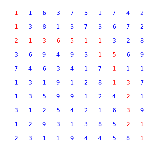
We iterate through all the points and labels (zipping them together for convenience), and then add a red text label if the point is in the path, or a blue label if it’s not.

Here’s what the visualisation looks like with the sample data:

Chiton Maze Path

Part 2

Urgh.

Now we’re told the cave is five times larger than our input data, in both the x and y dimensions. Thus, a total area 25x larger. We’re told our input data is actually just the first tile in a 5x5 grid of contiguous tiles. With each tile in either the x or y direction, the location risk is 1 higher than the risk level at the same position in the tile to the left or above (respectively).

Uber Grid

As before, we need to find the path from the top left to bottom right.

Our approach to Part 2 is as follows:

Update the Grid class so that it knows how to increment all its risk values. We’ll use this as we bolt on adjacent tiles.
Update the Grid class so that it knows how to stich on a new grid to the right.
Compute the 9 different grids we can make, by incrementing risk scores of our original grid. Since each location can only have a score 1 through 9, there are only 9 possible variants.
Stitch tiles to the right, to make a row 5 tiles wide.
Add “uber rows” of tiles below.
Finally, repeat our Dijkstra, using our much larger array.

In our Grid class, we only need to add the following:

    def increment_grid(self):
        """ Increment the value of every point in the array by 1.
        However, max is 9, and values wrap around to 1, NOT 0. """
        for point in self.all_points():
            value = self.value_at_point(point)
            if value < 9:
                self.set_value_at_point(point, value+1)
            else:
                self.set_value_at_point(point, 1)

    def append_grid(self, adjacent_grid: Grid) -> Grid:
        """ Append the new grid to the right of this grid.
        This creates a new grid which is horizontally bigger.
        Returns the new grid """

        this_array = self.array
        other_array = adjacent_grid.array
        
        new_rows = []
        for y in range(self.y_size):
            new_rows.append(this_array[y] + other_array[y])
            
        return Grid(new_rows)

The first method is pretty self-explanatory. It just increments every value in the grid, wrapping as required.
The append_grid() method bolts a new grid on to the right of this grid. It does this by concatenating each row in the two grids. Once done, it converts the list of str rows into a new Grid object.

Now we need to create our new 5x5 set of tiles, using our input data as the top left tile:

def build_uber_grid(start_grid: Grid, rows: int, cols:int) -> Grid:
    """ Build an uber grid, made up of y*x tiles, where each tile is the size of the start grid.
    With each tile to the right or down, all values increase by 1, according to increment rules. 
    """
    
    # Create the nine additional permutations of the starting tile 
    # (since each digit in the tile can only be from 1-9 inclusive)
    tile_permutations: dict[int, Grid] = {}
    tile_permutations[0] = start_grid
    for i in range(1, 9):
        tile = Grid(tile_permutations[i-1].array)
        tile.increment_grid()
        tile_permutations[i] = tile  # each tile is an increment of the grid before

    # Now stich each adjacent tile together to make an uber row            
    tile_rows: list[Grid] = []  # to hold y rows of very wide arrays
    for row in range(rows):
        tile_row = tile_permutations[row] # set the first tile in the row
        for col in range(1, cols):   # now add additional tiles to make the complete row
            tile_row = tile_row.append_grid(tile_permutations[row+col])
            
        tile_rows.append(tile_row)
    
    # now convert our five long grids into a single list of rows
    uber_rows = []
    for tile_row in tile_rows:
        for row in tile_row.array:
            uber_rows.append(row)
            
    return Grid(uber_rows)   

Finally, let’s run it:

# Part 2
# Build a new grid, which is 5x5 extension of our existing grid
uber_grid = build_uber_grid(grid, 5, 5)
path = navigate_grid(uber_grid) # Re-run our search
total_risk = sum([location[1] for location in path])
logger.info("Part 2 total risk: %d", total_risk)

And the output looks something like this:

44:02.345:INFO:__main__:     Part 1 total risk: 619
44:11.259:INFO:__main__:     Part 2 total risk: 2922
44:11.262:INFO:__main__:     Execution time: 2.2146 seconds

Onwards!

‹›