Advent of Code 2025 - Day 7

Useful Links

Concepts and Packages Demonstrated

Classes NamedTuple Recursion Shortest Paths (BFS)Memoization Graphs

Problem Intro

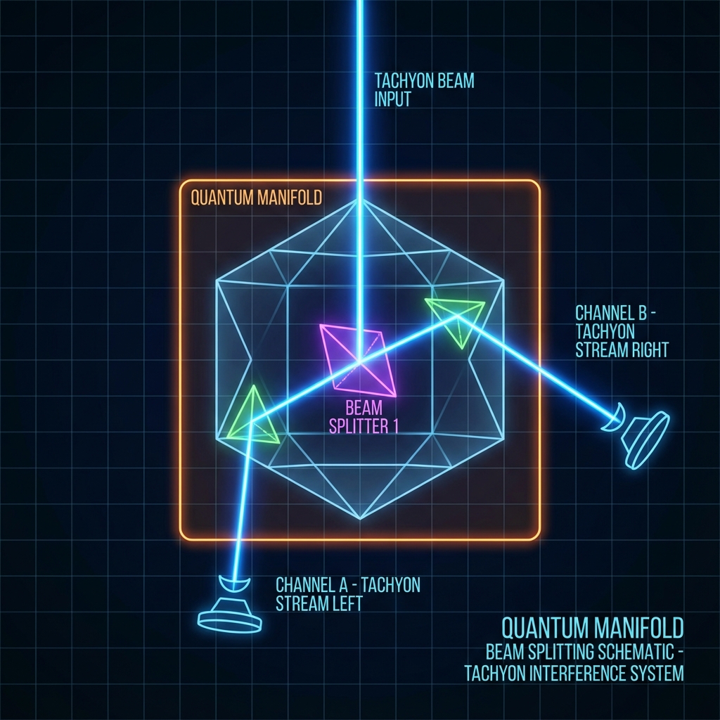
So… we’ve just teleported into a room, and — in classic Advent of Code fashion — we’re stuck! The room has no exits. But there is a broken teleporter that we need to fix. The room is a teleporter lab, and the broken part is a "Quantum Tachyon Manifold". (Sounds expensive, right?)

The puzzle asks us to simulate beams of tachyon particles moving through the manifold. The manifold schematic is our puzzle input, and it looks something ike this:

.......S.......
...............
.......^.......
...............
......^.^......
...............
.....^.^.^.....
...............
....^.^...^....
...............
...^.^...^.^...
...............
..^...^.....^..
...............
.^.^.^.^.^...^.
...............

S is the start of the beam. Beams always move downward, but they encounter splitters ^ which cause them to split into two separate beams (left-down and right-down). Beams pass through empty space.

Part 1

How many times will the beam be split?

Solution Walkthrough

1. Reusing the Grid

This problem is a classic grid traversal. I reused my Point named tuple and basic grid parsing logic from similar problems (like Day 4).

I chose NamedTuple for the Point class. Why? Because we are going to be creating a lot of points. NamedTuple is lightweight and immutable, making it memory efficient and hashable, so it can be used as a dictionary key or in a set.

Also, unlike standard tuples where you have to use confusing indices like point[0], NamedTuple gives us nice, readable dot notation like point.x and point.y.

class Point(NamedTuple):
    x: int
    y: int

My TachyonGrid class wraps the 2D list of characters and provides helper methods like valid_location(point) and value_at_point(point). Encapsulating this logic keeps the main solver clean.

2. BFS Simulation

For Part 1, we just need to count the splits. Since “merged” beams should not be double-counted, this is a standard Breadth-First Search (BFS).

We use a deque (double-ended queue) for our queue and a set for visited locations (explored).

deque: We can pop from the left side (popleft()) in O(1) time. A standard Python list pop(0) is O(n) because all remaining elements must shift. This efficiency is critical for BFS.
set: Checking if point in explored is O(1) on average. A list would be O(n), killing performance.

queue = deque([start])
explored = {start}
splits = 0

while queue:
    current = queue.popleft()
    if grid.value_at_point(current) == '^':
        splits += 1
        # Add new points (left and right) to queue IF not already explored
    else:
        # Add down point to queue IF not already explored

By adding to the explored set, we ensure we don’t process the same coordinate twice, effectively handling the “merging” rule.

Part 2: The Quantum Challenge

The manifold turns out to be quantum! There is only one particle, but every time it hits a splitter, it creates a new timeline! This means we need to track unique timelines. Even if two timelines end up at the same location, if they took different paths, they are distinct. We need to count the total number of timelines.

Part 2 removes the merging rule because every split creates a new timeline. If we just ran the Part 1 BFS without the explored set, the number of items in the queue would explode exponentially (2^n where n is split depth). This effectively becomes a Directed Acyclic Graph (DAG) of all possible paths.

The solution is Recursion with Memoization.

What is Memoization?

Memoization is just a fancy word for “caching the results of function calls”. If we invoke a function with specific arguments (e.g. count_timelines(Point(5, 5))), we calculate the result once and store it. If we ever call the function with those same arguments again, we return the stored result immediately.

This turns our exponential “tree” of paths into a linear scan of the grid. We only ever calculate the “future” of a specific grid point once.

Implementing DFS

Depth-First Search (DFS) can be implemented in two main ways:

Iterative: Using an explicit stack (LIFO data structure). You push items to the stack and pop from the top.
Recursive: Using the call stack implicitly. When a function calls itself, the current state is paused (pushed to the call stack), and the new call runs.

Recursion is often cleaner for graph traversals where we need to sum results from children (like “return left + right”). With an iterative stack, managing the return values from children back to parents can be messy.

Since the beams always move down (y increases), there are no loops. This makes it perfect for a recursive Depth-First Search (DFS). We define a function count_timelines(point) that answers: “If I am at this point, how many completed timelines will result?”

Base Case: If I’m off the grid, I’ve finished one valid timeline. Return 1.
Recursive Step:
- If I’m at a ^: result is count_timelines(left) + count_timelines(right).
- Otherwise: result is count_timelines(down).

Crucially, we use the @cache decorator from functools. This memoizes the result. If we ask for count_timelines at point (5, 10) and we’ve already calculated it (perhaps from a different timeline branch merging into this spot), we return the cached answer instantly.

I defined count_timelines as an inner function inside part2. This has several benefits:

Scope: It has access to the grid variable from the outer scope, so we don’t need to pass grid as an argument every time.
Encapsulation: The helper function is only relevant to part2, so keeping it inside keeps the global namespace clean.
Caching: We can easily apply @cache to this specific instance of the solver.

@cache
def count_timelines(point: Point) -> int:
    if not grid.valid_location(point):
        return 1

    val = grid.value_at_point(point)
    if val == '^':
        # Split! Sum the timelines from both branches
        return (count_timelines(Point(point.x - 1, point.y + 1)) + 
                count_timelines(Point(point.x + 1, point.y + 1)))
    else:
        # Continue specific timeline
        return count_timelines(Point(point.x, point.y + 1))

This transforms an exponential problem into a linear one (linear to the size of the grid).

Reflecting on this…

Honestly, I used to be terrified of recursion. The whole “function calling itself” thing melted my brain. But once you realise it’s just a way of saying “solve this small bit, then ask the same question for the next bit”, it clicks.

And functools.cache? Absolute game changer. It turns 20 lines of manual dictionary management into one line of code. Power-up!

Results

The final output looks something like this:

Part 1 soln=2591
Part 2 soln=31561750188661

The Part 2 solution is massive (20 trillion!), proving that a brute-force simulation would never have finished. But with memoization, it runs in 0.008 seconds.

‹›