The Python Journey - Visualisations and Plots with Matplotlib

‹›

Useful Links

MatplotlibOfficial Matplotlib TutorialsGeeks-for-Geeks Matplotlib TutorialGraph Plotting with MatplotlibPython Guides Matplotlib TutorialsImproving Your GraphsSeabornNumPy

Page Contents

• Overview
• Installing
• Basic Usage
  • Getting Axes
  • Showing the Visualisation
  • Grid Lines and Axis Limits
  • Saving the Visualisation to a File
• Examples
  • Basic Line Plot
  • Line Plots with Equations
  • Argand Diagram
  • Scatter Plot: No Lines
  • Inverted and With Hidden Axes: Rendering Characters!
  • Rendering Cubes using Matplotlib and NumPy
  • Rendering 3D Conway Cubes Animation, With NumPy and 3D Scatter
  • 2D Hexagons Animation
  • 2D Migration Animation
  • Rendering an Animated Snake with Scatter
  • Visualising a Path Through a Maze
  • Another Grid Visualisation
  • Plotting Trajectories
  • Plotting 3D Beacons
  • Plotting a 2D grid from NumPy, with Legend
  • Plotting and Filling a Polygon
  • Plotting a Perimeter and Marking Contained Points
  • Creating Squares Around Points
• Animating with Matplotlib
• Seaborn

Overview

Matplotlib is an amazing library for creating static, animated and interactive visualisations in Python, including graphs and 3D plots.

Installing

py -m pip install matplotlib

Basic Usage

• Many of the basic capabilities you’ll need are exposed through the pyplot. So the first thing you’ll want to do is import pyplot.
• Visualisations are created on figures, which in turn contain one more more axes; i.e. an individual plot area.

Getting Axes

Here are a few ways to obtain axes for plotting on:

from matplotlib import pyplot as plt

fig, axes = plt.subplots()

# or with 'get current axes'
axes = plt.gca()

# to set all axes to use equal aspects, rather than auto...
axes.set_aspect('equal', adjustable='box')

Showing the Visualisation

# To show interactively, i.e. pausing code execution until the window is closed
plt.show()

Grid Lines and Axis Limits

# add grid lines
axes.grid(True)

# set the limits for each axis
axes.set_xlim(-4, 4)
axes.set_ylim(-4, 4)
axes.set_xlabel("real")
axes.set_ylabel("imag")

plt.show()

The output looks like this:

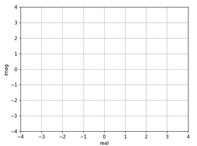
Of course, there’s no data yet.

Saving the Visualisation to a File

Instead of rendering the visualisation interactively, we can instead save it. This is easy to do. Instead of using plt.show(), we use plt.savefig() and pass in the file we want to save to.

# Save visualisation to a file
plt.savefig("myfile.jpg")

# With a transparent background
plt.savefig("myfile.jpg", transparent=True)

Maybe we want to save to a particular folder, and create that folder if it doesn’t already exit:

from pathlib import Path

SCRIPT_DIR = Path(__file__).parent            # working directory
OUTPUT_DIR = Path(SCRIPT_DIR, "output/")      # where we want to put our new file
OUTPUT_FILE = Path(OUTPUT_DIR, "my_vis.png")  # the name of our new file

if not Path.exists(OUTPUT_DIR):               # Create folder if it doesn't exist
    Path.mkdir(OUTPUT_DIR)
plt.savefig(OUTPUT_FILE)

Examples

The next few examples will start with this:

from matplotlib import pyplot as plt

fig, axes = plt.subplots()

# add grid lines
axes.grid(True)
axes.set_xlabel("x")
axes.set_ylabel("y")

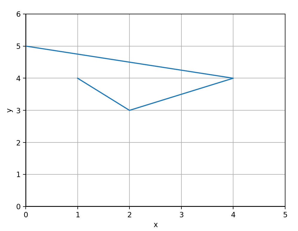
Basic Line Plot

# create list of points
points = [ (1, 4), (2, 3), (4, 4), (0, 5) ]

# Unpack our x, y vals
all_x, all_y = zip(*points)

# Create out axes
fig, axes = plt.subplots()

# add lines at x=0, y=0 and labels
plt.axhline(0, color='black')
plt.axvline(0, color='black')
axes.set_xlim(0, max(all_x)+1)
axes.set_ylim(0, max(all_y)+1)
axes.set_xlabel("x")
axes.set_ylabel("y")

# add grid lines
axes.grid(True)

plt.plot(all_x, all_y)
plt.show()

Output:

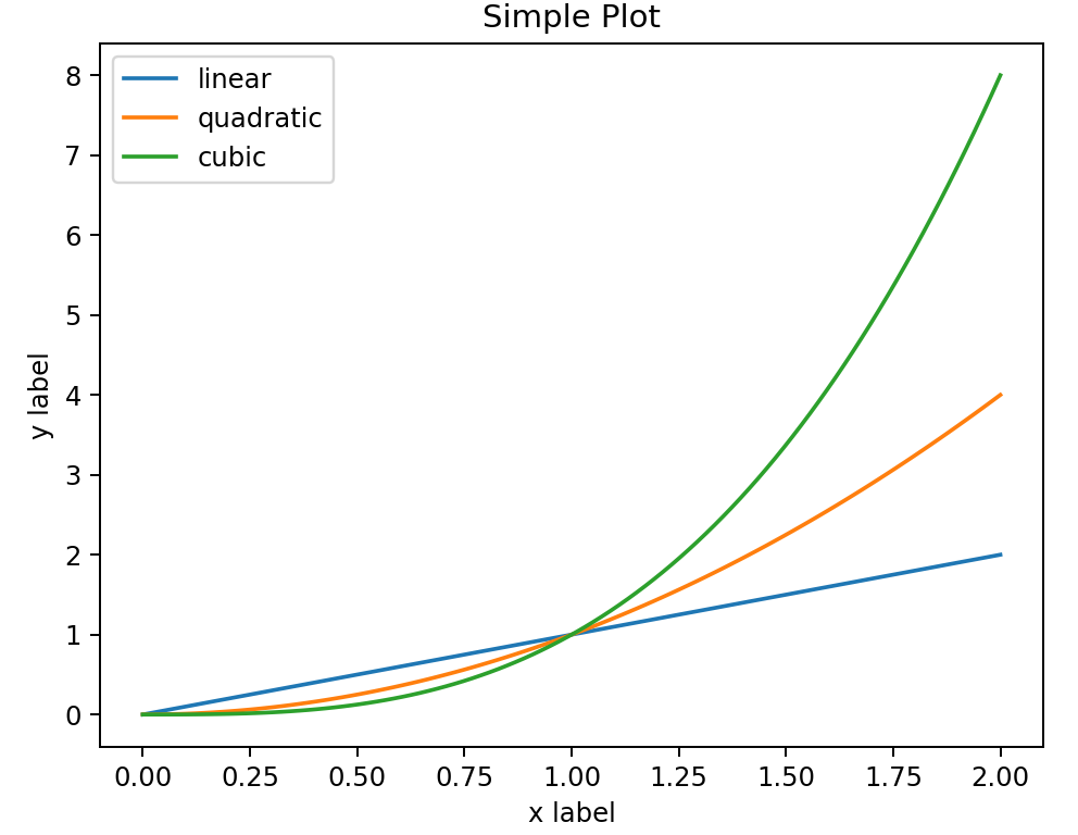
Line Plots with Equations

x = np.linspace(0, 2, 100) # Generate a numpy array of data to plot

fig, ax = plt.subplots()  # Create a figure and an axes
ax.plot(x, x, label='linear')  # Plot some data on the axes
ax.plot(x, x**2, label='quadratic')  # Plot more data on the axes...
ax.plot(x, x**3, label='cubic')  # ... and some more.
ax.set_xlabel('x label')  # Add an x-label to the axes.
ax.set_ylabel('y label')  # Add a y-label to the axes.
ax.set_title("Simple Plot")  # Add a title to the axes.
ax.legend()  # Add a legend.

plt.show()

Output:

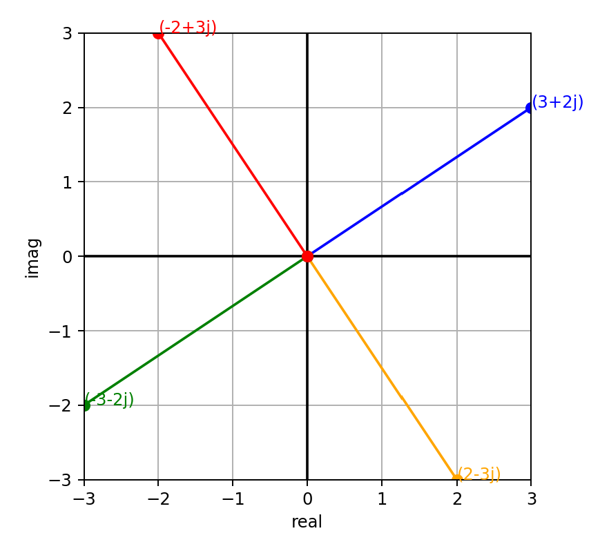
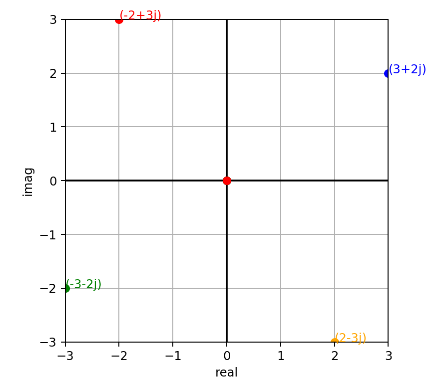
Argand Diagram

def cw_rotate(z: complex, degrees: float) -> complex:
    """ Returns a new point, after rotating the supplied point about the origin, clockwise.

    Args:
        z (complex): Point to rotate
        degrees (float): Degrees to rotate, CW

    Returns:
        complex: A new points
    """
    # Note that complex number phase is expressed as a CCW angle to the real axis.
    # Thus, to rotate CW, we have to always take the supplied angle from 360.
    return z * 1j**((360-degrees)/90)

points: list[complex] = [] # store our points

POINT = 3+2j # starting point
print(POINT)
points.append(POINT)

for cw_angle in (90, 180, 270):
    rotated_point = cw_rotate(POINT, cw_angle)
    points.append(rotated_point)

fig, axes = plt.subplots()  # Create out axes
axes.set_aspect('equal') # set x and y to equal aspect
axes.grid(True) # add grid lines

# add lines at x=0, y=0
plt.axhline(0, color='black')
plt.axvline(0, color='black')

# set the limits and labels for each axis
all_x = [num.real for num in points]
all_y = [num.imag for num in points]
axes.set_xlim(min(all_x), max(all_x))
axes.set_ylim(min(all_y), max(all_y))
axes.set_xlabel("real")
axes.set_ylabel("imag")

colours = ['blue', 'orange', 'green', 'red']

# Iterate over each point and plot
for i, point in enumerate(points):
    # For this point, plot from origin to the point
    plt.plot([0, point.real], [0, point.imag], '-', marker='o', color=colours[i])
    
    # Add an annotation to the point.  We can do this one of two ways...
    # plt.text(point.real, point.imag, str(point))
    plt.annotate(str(point), (point.real, point.imag), color=colours[i])
    
plt.show()

Output:

Scatter Plot: No Lines

We can amend one line above and use the format string parameter to remove the lines, as follows:

plt.plot([0, point.real], [0, point.imag], 'o', color=colours[i])

Inverted and With Hidden Axes: Rendering Characters!

Imagine we have a number of (x,y) coordinates defined in a set of point objects called dots. We can render them in a cool way, like this:

""" Render these coordinates as a scatter plot """
all_x = [point.x for point in dots]
all_y = [point.y for point in dots]

axes = plt.gca()
axes.set_aspect('equal')
plt.axis("off") # hide the border around the plot axes
axes.set_xlim(min(all_x)-1, max(all_x)+1)
axes.set_ylim(min(all_y)-1, max(all_y)+1)
axes.invert_yaxis()

axes.scatter(all_x, all_y, marker="o", s=50)
plt.show()

Output:

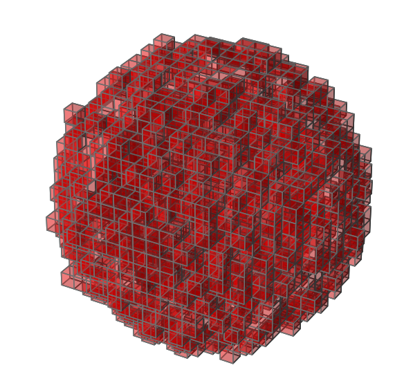
Rendering Cubes Using Matplotlib and NumPy

Here’s an example that renders 3D cubes based on a set of 3D coordinates:

    def vis(self):
        """ Render a visualisation of our droplet """

        axes = [self._max_x+1, self._max_y+1, self._max_z+1]  # set bounds
        grid = np.zeros(axes, dtype=np.int8)   # Initialise 3d grid to empty
        for point in self.filled_cubes:  # set our array to filled for all filled cubes
            grid[point.x, point.y, point.z] = 1
        
        facecolors = np.where(grid==1, 'red', 'black')
        
        # Plot figure
        fig = plt.figure()
        ax = fig.add_subplot(111, projection='3d')
        ax.voxels(grid, facecolors=facecolors, edgecolors="grey", alpha=0.3)
        ax.set_aspect('equal')
        plt.axis("off")
        plt.show()

The code above is taken from my 2022 Day 18 solution. The rendered image looks like this:

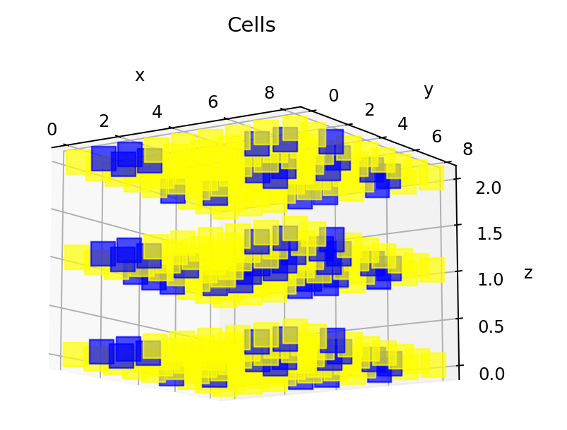
Rendering 3D Conway Cubes Animation, With NumPy and 3D Scatter

Taken from 2020 Day 17: Conway Cubes:

def show_grid(grid):
    x_vals = [cell.get_x() for cell in grid]
    y_vals = [cell.get_y() for cell in grid]
    z_vals = [cell.get_z() for cell in grid]

    min_x_add = 0
    min_y_add = 0
    min_z_add = 0

    min_x = min(x_vals)
    min_y = min(y_vals)
    min_z = min(z_vals)

    # we need to get rid of negative coords, since numpy doesn't support -ve values for indexes
    if min_x < 0:
        min_x_add = 0 - min_x
    if min_y < 0:
        min_y_add = 0 - min_y
    if min_z < 0:
        min_z_add = 0 - min_z        

    x_size = (max(x_vals) + 1) - min(x_vals)
    y_size = (max(y_vals) + 1) - min(y_vals)
    z_size = (max(z_vals) + 1) - min(z_vals)
    xyz = np.zeros((x_size, y_size, z_size))
    for cell in grid:
        x = cell.get_x() + min_x_add
        y = cell.get_y() + min_y_add
        z = cell.get_z() + min_z_add

        xyz[x, y, z] = 1

    axes = plt.axes(projection='3d')
    for index, active in np.ndenumerate(xyz):
        if active == 1:
            axes.scatter3D(*index, c='blue', marker='s', s=200, alpha=0.7)
        else:
            axes.scatter3D(*index, c='yellow', marker='s', s=200, alpha=0.7)

    axes.set_xlabel('x')
    axes.set_ylabel('y')
    axes.set_zlabel('z')
    axes.set_title('Cells')

    plt.show()

2D Hexagons Animation

Taken from 2020 Day 24: Hexagons and Neighbours:

def vis_state(black_tiles, all_tiles, iteration):
    white_tiles = all_tiles.difference(black_tiles)

    all_x, all_y = zip(*all_tiles)
    white_x, white_y = zip(*white_tiles)
    black_x, black_y = zip(*black_tiles)
    
    min_x, max_x = min(all_x), max(all_x)
    min_y, max_y = min(all_y), max(all_y)

    # hexagon!
    shape = 'h'

    fig, ax = plt.subplots(dpi=141)
    ax.set_facecolor('xkcd:orange')
    ax.set_xlim(min_x-1, max_x+1)
    ax.set_ylim(min_y-1, max_y+1)

    # we want x axis compressed, given our hex geometry.
    # I.e. given that e or w = 2 units.
    ax.set_aspect(1.75)

    # dynamically compute the marker size
    fig.canvas.draw()
    mkr_size = ((ax.get_window_extent().width / (max_x-min_x) * (134/fig.dpi)) ** 2)

    # make sure the ticks have integer values
    ax.xaxis.set_major_locator(MaxNLocator(integer=True))
    
    ax.scatter(black_x, black_y, marker=shape, s=mkr_size, color='black', edgecolors='black')
    ax.scatter(white_x, white_y, marker=shape, s=mkr_size, color='white', edgecolors='black')
    ax.set_title(f"Tile Floor, Iteration: {iteration-1}")
    
    if not os.path.exists(OUTPUT_DIR):
        os.makedirs(OUTPUT_DIR)

    # save the plot as a frame
    filename = OUTPUT_DIR + "tiles_anim_" + str(iteration) + ".png"
    plt.savefig(filename)
    # plt.show()
    anim_frame_files.append(filename)

2D Migration Animation

Taken from 2021 Day 25: Migrating Sea Cucumbers:

    def _render_frame(self):
        """ Only renders an animation frame if we've attached an Animator """
        if not self._animator:
            return
        
        east = set()
        south = set()
        
        for y in range(self._grid_len):
            for x in range(self._row_len):
                if self._grid[y][x] == ">":
                    east.add((x,y))
                elif self._grid[y][x] == "v":
                    south.add((x,y))
        
        east_x, east_y = zip(*east)
        south_x, south_y = zip(*south)
        
        axes, mkr_size = self._plot_info
        
        axes.clear()
        min_x, max_x = -0.5, self._row_len - 0.5
        min_y, max_y = -0.5, self._grid_len - 0.5
        axes.set_xlim(min_x, max_x)
        axes.set_ylim(max_y, min_y)
        
        axes.scatter(east_x, east_y, marker=">", s=mkr_size, color="black")
        axes.scatter(south_x, south_y, marker="v", s=mkr_size, color="white")
        
        # save the plot as a frame; store the frame in-memory, using a BytesIO buffer
        frame = BytesIO()
        plt.savefig(frame, format='png') # save to memory, rather than file
        self._animator.add_frame(frame)

    def setup_fig(self):
        if not self._animator:
            return
        
        my_dpi = 120
        fig, axes = plt.subplots(figsize=(1024/my_dpi, 768/my_dpi), dpi=my_dpi, facecolor="black") # set size in pixels

        axes.get_xaxis().set_visible(False)
        axes.get_yaxis().set_visible(False)
        axes.set_aspect('equal') # set x and y to equal aspect
        axes.set_facecolor('xkcd:orange')
        
        min_x, max_x = -0.5, self._row_len - 0.5
        min_y, max_y = -0.5, self._grid_len - 0.5
        axes.set_xlim(min_x, max_x)
        axes.set_ylim(max_y, min_y)

        # dynamically compute the marker size
        fig.canvas.draw()
        mkr_size = ((axes.get_window_extent().width / (max_x-min_x) * (45/fig.dpi)) ** 2)
        return axes, mkr_size

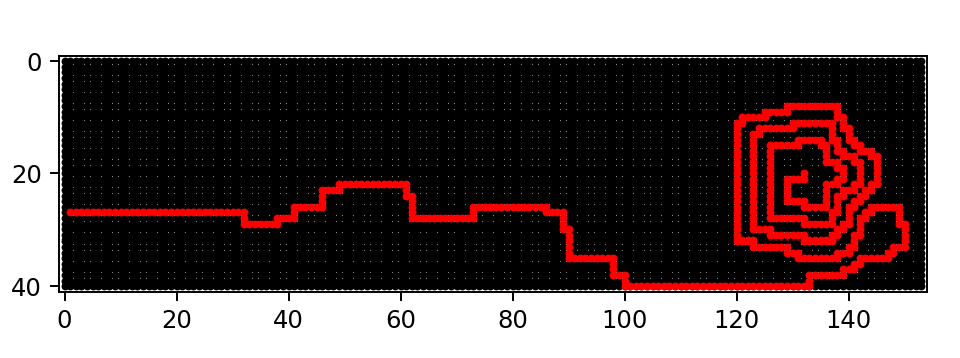
Rendering an Animated Snake with Scatter

Taken from 2022 Day 09 - Rope Bridge:

    def _init_plt(self):
        """ Generate a Figure and Axes objects which are reused. """
        my_dpi = 120
        figure, axes = plt.subplots(figsize=(1024/my_dpi, 768/my_dpi), dpi=my_dpi, facecolor="white") # set size in pixels
        axes.set_aspect('equal') # set x and y to equal aspect
        axes.set_facecolor('xkcd:black')
        
        return figure, axes
    
    def _render_frame(self, visited: set[Point], iteration: int=0):
        """ Only renders an animation frame if we've attached an enabled Animator """
        
        fig, axes = self._plt_info
        axes.clear()
        
        # The grid will grow as the rope heads moves around
        max_x = max(self._all_head_locations, key=lambda point: point.x).x
        min_x = min(self._all_head_locations, key=lambda point: point.x).x
        max_y = max(self._all_head_locations, key=lambda point: point.y).y
        min_y = min(self._all_head_locations, key=lambda point: point.y).y
        axes.set_xlim(min_x - 2, max_x + 2)
        axes.set_ylim(min_y - 2, max_y + 2)

        # dynamically compute the marker size
        fig.canvas.draw()
        factor = 40  # Smaller factor means smaller markers
        mkr_size = int((axes.get_window_extent().width / (max_x-min_x+1) * (factor/fig.dpi)) ** 2)

        # make sure the ticks have integer values
        axes.xaxis.set_major_locator(MaxNLocator(integer=True))
        
        head = self._knots[0]
        tail = self._knots[-1]
        others_knots = self._knots[1:-1]
        
        visited_x = [point.x for point in visited if point != tail]
        visited_y = [point.y for point in visited if point != tail]

        for knot in others_knots:
            axes.scatter(knot.x, knot.y, marker=MarkerStyle("."), s=mkr_size/2, color="white")
            
        axes.scatter(head.x, head.y, marker=MarkerStyle("."), s=mkr_size, color="red")
        axes.scatter(visited_x, visited_y, marker=MarkerStyle("x"), s=mkr_size/3, color="grey")
        axes.scatter(tail.x, tail.y, marker=MarkerStyle("*"), s=mkr_size/2, color="yellow")
                
        axes.set_title(f"Iteration: {iteration}; tail has visited {len(visited)} locations")
        
        # save the plot as a frame; store the frame in-memory, using a BytesIO buffer
        frame = BytesIO()
        plt.savefig(frame, format='png') # save to memory, rather than file
        self._animator.add_frame(frame)

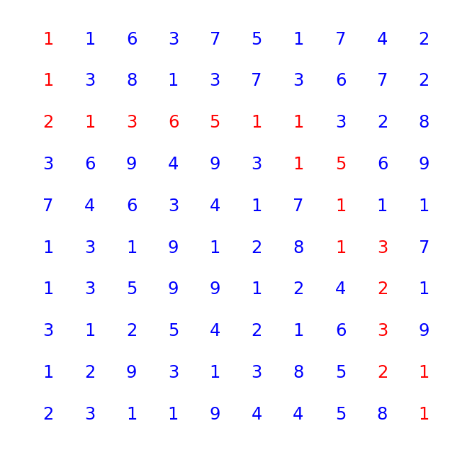
Visualising a Path Through a Maze

Taken from 2021 Day 15: Risk Maze:

def visualise_path(grid: Grid, path: list[tuple[Point, int]]):
    """ Render this paper and its dots as a scatter plot """
    all_x = [point.x for point in grid.all_points()]
    all_y = [point.y for point in grid.all_points()]
    labels = [grid.value_at_point(point) for point in grid.all_points()]
    path_points = [Point(0,0)] + [path_item[0] for path_item in path]
    
    axes = plt.gca()
    axes.set_aspect('equal')
    plt.axis("off") # hide the border around the plot axes
    axes.set_xlim(min(all_x)-1, max(all_x)+1)
    axes.set_ylim(min(all_y)-1, max(all_y)+1)
    axes.invert_yaxis()
    
    for point, label in zip(grid.all_points(), labels):
        if point in path_points:
            plt.text(point.x, point.y, s=str(label), color="r")
        else:
            plt.text(point.x, point.y, s=str(label), color="b")
        
    plt.show()

Another Grid Visualisation

Taken from 2022 Day 12: Hill Climbing:

def render_as_plt(grid, path):
    """ Render the display as a scatter plot """  
    x_vals = [point.x for point in grid.all_points()]
    y_vals = [point.y for point in grid.all_points()]
    
    path_x = [point.x for point in path]
    path_y = [point.y for point in path]
    
    axes = plt.gca()
    axes.set_aspect('equal')
    axes.set_xlim(min(x_vals)-1, max(x_vals)+1)
    axes.set_ylim(min(y_vals)-1, max(y_vals)+1)
    axes.invert_yaxis()
    
    axes.scatter(x_vals, y_vals, marker="o", s=5, color="black")
    axes.scatter(path_x, path_y, marker="o", s=5, color="red")
    plt.show()    

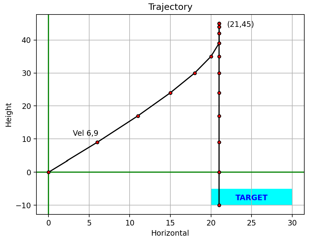
Plotting Trajectories

Taken from 2021 Day 17: Probe Trajectories:

def plot_trajectory(trajectory: list[Point], target: Rect, outputfile=None):
    """ Render this trajectory as a plot, and optionally save it """
    axes = plt.gca()
    
    # Add axis lines at x=0 and y=0
    plt.axhline(0, color='green')
    plt.axvline(0, color='green') 
    axes.grid(True) # grid lines on
    
    # Set up titles
    axes.set_title("Trajectory")
    axes.set_xlabel("Horizontal")
    axes.set_ylabel("Height")
    
    axes.fill(*target.as_polygon(), 'cyan')  # add the target area
    plt.annotate("TARGET", (target.left_x, target.top_y), 
                 xytext=(target.left_x + ((target.right_x - target.left_x)/2)-2, 
                        (target.top_y - (target.top_y-target.bottom_y)/2)-1), 
                 color="blue", weight='bold') 
    
    # Plot the trajectory points
    all_x = [point.x for point in trajectory]
    all_y = [point.y for point in trajectory]
    plt.plot(all_x, all_y, marker="o", markerfacecolor="red", markersize=4, color='black')
    
    x, y = trajectory[1].x, trajectory[1].y
    plt.annotate(f"Vel {x},{y}", (x,y), xytext=(x-3, y+2))  # label first point
    x, y = [(point.x, point.y) for point in trajectory if point.y == max(point.y for point in trajectory)][0]
    plt.annotate(f"({x},{y})", (x,y), xytext=(x+1, y-1))  # label highest point    
        
    if outputfile:
        dir_path = Path(outputfile).parent
        if not Path.exists(dir_path):
            Path.mkdir(dir_path)
        plt.savefig(outputfile)
        logger.info("Plot saved to %s", outputfile)        
    else:
        plt.show()

Plotting 3D Beacons

Taken from 2021 Day 19: Beacons and Scanners:

def plot(scanner_locations: dict[int, Vector], beacon_locations: set[Vector], outputfile=None):
    _ = plt.figure(111)
    axes = plt.axes(projection="3d")
    axes.set_xlabel("x")
    axes.set_ylabel("y")
    axes.set_zlabel("z")

    axes.grid(True) # grid lines on
    
    x,y,z = zip(*scanner_locations.values())    # scanner locations
    axes.scatter3D(x, y, z, marker="o", color='r', s=40, label="Sensor")
    offset=50
    for x, y, z, scanner in zip(x, y, z, scanner_locations.keys()): # add scanner numbers
        axes.text3D(x+offset, y+offset, z+offset, s=scanner, color="red", fontweight="bold")
    
    x,y,z = zip(*beacon_locations)
    axes.scatter3D(x, y, z, marker=".", c='blue', label="Probe", s=10)
    
    x_line = [min(x), max(x)]
    y_line = [0, 0]
    z_line = [0, 0]
    plt.plot(x_line, y_line, z_line, color="black", linewidth=1)
    
    x_line = [0, 0]
    y_line = [min(y), max(y)]
    z_line = [0, 0]
    plt.plot(x_line, y_line, z_line, color="black", linewidth=1)
    
    x_line = [0, 0]
    y_line = [0, 0]
    z_line = [min(z), max(z)]
    plt.plot(x_line, y_line, z_line, color="black", linewidth=1)
    
    axes.legend()
    plt.title("Scanner and Beacon Locations", fontweight="bold")

    if outputfile:
        dir_path = Path(outputfile).parent
        if not Path.exists(dir_path):
            Path.mkdir(dir_path)
        plt.savefig(outputfile)
        logger.info("Plot saved to %s", outputfile)        
    else:
        plt.show()

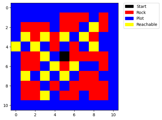
Plotting a 2D grid from NumPy, with Legend

Sometimes it can be more effective to convert a 2D array into NumPy format before plotting. E.g.

Taken from 2023 Day 21: Finding Paths:

def plot(grid, start, visited: set):
    # Map the characters to numbers: S -> 0, # -> 1, . -> 2, O -> 3
    char_to_num = {'S': 0, '#': 1, '.': 2, 'O': 3}
    cmap = mcolors.ListedColormap(['black', 'red', 'blue', 'yellow'])
    numeric_grid = [[char_to_num[char] for char in row] for row in grid]
        
    # Convert to a NumPy array for better handling by Matplotlib
    numeric_grid = np.array(numeric_grid)

    for (ci,ri) in visited: # update visited
        numeric_grid[ri][ci] = 3
    numeric_grid[start[1],start[0]] = 0 # update start
    
    # Create custom patches for the legend
    labels = ['Start', 'Rock', 'Plot', 'Reachable']
    colors = ['black', 'red', 'blue', 'yellow']
    patches = [mpatches.Patch(color=colors[i], label=labels[i]) for i in range(len(colors))]

    plt.imshow(numeric_grid, cmap=cmap)
    plt.legend(handles=patches, bbox_to_anchor=(1.05, 1), loc=2, borderaxespad=0.)
    plt.show()

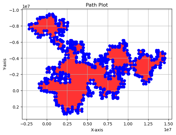
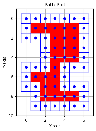
Plotting and Filling a Polygon

Taken from 2023 Day 18: Filling the Lava Lagoon:

def plot_path(perimeter: list[tuple]):
    # Extract x and y values from the perimeter
    perimeter_x_values = [point[0] for point in perimeter]
    perimeter_y_values = [point[1] for point in perimeter]
    
    # Plot the perimeter as a line
    plt.plot(perimeter_x_values, perimeter_y_values, 
             marker=MarkerStyle('o'), linestyle='-', color="blue", label="Perimeter")

    # Fill the inside of the perimeter
    plt.fill(perimeter_x_values, perimeter_y_values, color="red", alpha=0.8)  # Adjust alpha for transparency

    plt.title('Path Plot')
    plt.xlabel('X-axis')
    plt.ylabel('Y-axis')
    plt.gca().invert_yaxis()  # Invert the y-axis
    plt.gca().set_aspect('equal', adjustable='box')  # Set equal scale 
    plt.grid(True)
    plt.show()

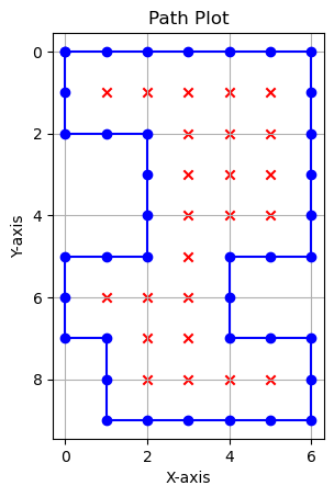
Plotting a Perimeter and Marking Contained Points

Taken from 2023 Day 18: Filling the Lava Lagoon:

def plot_path(path: list[tuple], inside: set[tuple]=set()):
    # Extract x and y values from the path
    loop_x_values = [point[0] for point in path]
    loop_y_values = [point[1] for point in path]
    
    # Extract x and y values from the inside set
    inside_x_values = [point[0] for point in inside]
    inside_y_values = [point[1] for point in inside]

    # Plot the line and scatter graphs
    plt.plot(loop_x_values, loop_y_values, 
             marker=MarkerStyle('o'), linestyle='-', color="blue", label="Loop")
        
    plt.scatter(inside_x_values, inside_y_values, 
                marker=MarkerStyle('x'), color="red", label="Inside")
    
    plt.title('Path Plot')
    plt.xlabel('X-axis')
    plt.ylabel('Y-axis')
    plt.gca().invert_yaxis()  # Invert the y-axis
    plt.gca().set_aspect('equal', adjustable='box') # set equal scale 
    plt.grid(True)
    plt.show()

Creating Squares Around Points

Taken from 2023 Day 18: Filling the Lava Lagoon:

def plot_path(path: list[tuple], inside: set[tuple]=set()):
    fig, ax = plt.subplots()

    # Function to add a 1x1 square with the point at its center
    def add_square(x, y, colour, fill=False):
        square = Rectangle((x - 0.5, y - 0.5), 1, 1, fill=fill, edgecolor=colour, facecolor=colour)
        ax.add_patch(square)

    # Plot each point in the path as a square
    for point in path:
        add_square(point[0], point[1], 'blue')

    # Plot each point in the inside set as a square
    for point in inside:
        add_square(point[0], point[1], 'red', fill=True)

    # Extract x and y values for vertices
    path_x_values = [point[0] for point in path]
    path_y_values = [point[1] for point in path]
    inside_x_values = [point[0] for point in inside]
    inside_y_values = [point[1] for point in inside]
    
    # Plot the actual vertex points
    ax.scatter(path_x_values, path_y_values, color="blue", zorder=5)
    ax.scatter(inside_x_values, inside_y_values, color="blue", zorder=5)
    
    # Set limits for x and y axis
    all_x_values = [point[0] for point in path] + [point[0] for point in inside]
    all_y_values = [point[1] for point in path] + [point[1] for point in inside]

    ax.set_xlim(min(all_x_values) - 1, max(all_x_values) + 1)
    ax.set_ylim(min(all_y_values) - 1, max(all_y_values) + 1)

    plt.title('Path Plot')
    plt.xlabel('X-axis')
    plt.ylabel('Y-axis')
    plt.gca().invert_yaxis()
    plt.gca().set_aspect('equal', adjustable='box')
    plt.grid(True)
    plt.show()

Animating with Matplotlib

E.g.

Taken from 2023 Day 16: Light Paths Through a Grid:

class LightGrid(Grid):
    """ Represents a 2D grid containing empty space (.), mirrors, and splitters (- and |).
    Light passes through empty space. Light is refracted by 90 degrees at a mirror. 
    Light is split in the two orthogonal directions at a splitter, or allowed to pass through unchanged, 
    depending on orientation. """
    
    MIRROR_DIRECTION_MAP = { # { (current char, current direction): new direction }
        ("/", Vectors.E.value): Vectors.N.value,
        ("/", Vectors.S.value): Vectors.W.value,
        ("/", Vectors.W.value): Vectors.S.value,
        ("/", Vectors.N.value): Vectors.E.value,
        ("\\", Vectors.E.value): Vectors.S.value,
        ("\\", Vectors.S.value): Vectors.E.value,
        ("\\", Vectors.W.value): Vectors.N.value,
        ("\\", Vectors.N.value): Vectors.W.value,
    }
    
    VECTORS_TO_ARROWS = { # used for rendering a console representation
        Vectors.N.value: "^",
        Vectors.E.value: ">",
        Vectors.S.value: "v",
        Vectors.W.value: "<",
    }
    
    def __init__(self, grid_array: list, animating: bool = False, **kwargs) -> None:
        """ Creates a grid that light beams pass through. """
       
        # [ (posn, dirn), ... ]
        # dirn is the direction we were facing when we arrived at this position
        self.path_taken: list[tuple[Point, tuple[int,int]]] = []
        self.energised = defaultdict(set) # { point: {dirn}, }
        super().__init__(grid_array=grid_array, animating=animating, **kwargs)
    
    def animate_step(self, i):
        """ Update the plot for the ith step in the animation. """
        if self._frame_index < len(self.path_taken):
            if self._frame_index % 100 == 0:
                logger.debug(f"Rendering frame {self._frame_index}")
                
            self._render_plot()
            self._frame_index += 1
        return []
    
    def create_animation(self, output_path='animation.mp4', fps=10):
        """ Create the animation, by calling the animate_step() method to generate frames. """
        self._plot_info = self._setup_fig()  # Set up the figure for plotting
        fig, axes, mkr_size = self._plot_info
        
        logger.debug(f"Creating the animation. We have {len(self.path_taken)} frames to render.")
        # Creating the animation
        anim = FuncAnimation(fig, self.animate_step, frames=len(self.path_taken), 
                             interval=1000/fps, blit=True)

        # Save the animation
        anim.save(output_path, writer='ffmpeg')
    
    def bfs(self, start:tuple[Point,tuple[int,int]]=(Point(0,0), Vectors.E.value)):
        """ Perform a BFS to build the path that light takes through the grid.

        Args:
            start (tuple, optional): (point, vector value). Defaults to (Point(0,0), Vectors.E
        """
        frontier = deque() # ideal for FIFO
        frontier.append(start)
        explored = set()
        explored.add(start)

        while frontier:
            posn, dirn = frontier.popleft() # point, vector value
            self.path_taken.append((posn, dirn))
            self.energised[posn].add(dirn)       
            
            for neighbour in self.next_move(posn, dirn):
                if self.valid_location(neighbour[0]): # is this next move in the grid?
                    if neighbour not in explored:
                        frontier.append(neighbour)
                        explored.add(neighbour)
    
    def next_move(self, posn:Point, dirn:tuple):
        """ Determine the next moves that are valid from here. Returns each move sequentially, as a generator.
        For any given current (point, direction), we can move to 1 or 2 adjacent points. 
        If the current point is a mirror, the new direction will be different.
        If the current point is a splitter, the new direction will be different if we've hit the splitter
        from a perpendicular direction.

        Args:
            posn (Point): Our current location
            dirn (Vector tuple): The direction we were facing when we landed at this point

        Yields:
            tuple: (next point, next direction)
        """

        curr_val = self.value_at_point(posn) # where are we now

        # First, check our "pass through" conditions...
        if (curr_val == "." or (curr_val == "|" and dirn in (Vectors.N.value, Vectors.S.value))
                            or (curr_val == "-" and dirn in (Vectors.E.value, Vectors.W.value))):
            next_dirn = dirn 
            next_posn = posn + Point(*next_dirn)
            yield (next_posn, dirn)            
        elif curr_val in ("/", "\\"): # Now map directions if we're at a mirror
            next_dirn = LightGrid.MIRROR_DIRECTION_MAP[(curr_val, dirn)]
            next_posn = posn + Point(*next_dirn)
            yield (next_posn, next_dirn)                      
        elif curr_val ==  "|": # split at |, yielding two directions
            assert dirn in (Vectors.E.value, Vectors.W.value), "We must be going E or W"
            for next_dirn in (Vectors.N.value, Vectors.S.value):
                next_posn = posn + Point(*next_dirn)
                yield (next_posn, next_dirn)
        else: # split at -, yielding two directions
            assert curr_val == "-", "We should be at -"
            assert dirn in (Vectors.N.value, Vectors.S.value), "We must be going N or S"
            for next_dirn in (Vectors.E.value, Vectors.W.value):
                next_posn = posn + Point(*next_dirn)
                yield (next_posn, next_dirn)                    
        
    def __str__(self) -> str:
        """ Generate a str representation of the grid, including the path_taken. """
        rows = []
        for row_num, row in enumerate(self.array):
            repr = []
            for char_num, char in enumerate(row):
                point = Point(char_num, row_num)
                if point in self.energised:
                    repr.append(Fore.YELLOW)
                    if char not in ("|", "-", "\\", "/"):
                        dirs_for_locn = len(self.energised[point])
                        if dirs_for_locn == 1:
                            dirn = list(self.energised[point])[0]
                            repr.append(LightGrid.VECTORS_TO_ARROWS[dirn])                   
                        else:
                            repr.append(str(dirs_for_locn))
                    else:
                        repr.append(char)
                    repr.append(Fore.RESET)
                else:
                    repr.append(char)
            
            rows.append("".join(repr))
        
        return "\n".join(rows)

    def _setup_fig(self):
        """ Initialise the plot """      
        my_dpi = 120
        fig, axes = plt.subplots(figsize=(1024/my_dpi, 768/my_dpi), dpi=my_dpi, facecolor="white") # set size in pixels

        axes.get_xaxis().set_visible(True)
        axes.get_yaxis().set_visible(True)
        axes.invert_yaxis()
        axes.set_aspect('equal') # set x and y to equal aspect
        axes.set_facecolor('xkcd:black')
        
        min_x, max_x = -0.5, self.width - 0.5
        min_y, max_y = -0.5, self.height - 0.5
        axes.set_xlim(min_x, max_x)
        axes.set_ylim(max_y, min_y)

        # dynamically compute the marker size
        fig.canvas.draw()
        mkr_size = ((axes.get_window_extent().width / (max_x-min_x) * (45/fig.dpi)) ** 2)
        return fig, axes, mkr_size
    
    def plot(self):
        """ Show the current plot """
        self._render_plot(frame_idx=-1)
        plt.show()
        
    def _render_plot(self, frame_idx=None):
        """ Add each new frame. Note that this method should draw should only draw up to a particular state. 
        If frame_idx is set, it will render the plot at that particular frame. Use -1 for final state. """
        fig, axes, mkr_size = self._plot_info
        axes.clear() # Clear the axes to start fresh for each frame
        axes.invert_yaxis()
       
        dir_sets = [set() for _ in range(4)]
            
        # Plot the path
        # Only plot the path up to the current frame index
        last_frame = frame_idx if frame_idx else (self._frame_index + 1)
        for point, dirn in self.path_taken[:last_frame]:
            for dir_set, arrow in zip(dir_sets, ("^", ">", "v", "<")):
                if LightGrid.VECTORS_TO_ARROWS[dirn] == arrow:
                    dir_set.add(point)
                    continue

        for dir_set, arrow in zip(dir_sets, ("^", ">", "v", "<")):
            if dir_set:
                dir_set_x, dir_set_y = zip(*((point.x, point.y) for point in dir_set))
                axes.scatter(dir_set_x, dir_set_y, marker=arrow, s=mkr_size*0.5, color="white")            

        # Plot the infra
        vert_splitters, horz_splitters, forw_mirrors, back_mirrors = set(), set(), set(), set()
        infra_mappings = {
            '|': vert_splitters, 
            '-': horz_splitters, 
            '/': forw_mirrors, 
            '\\': back_mirrors
        }
        
        for row_num, row in enumerate(self.array):
            for char_num, char in enumerate(row):
                point = Point(char_num, row_num)
                if char in infra_mappings:
                    infra_mappings[char].add(point)        
                    
        for infra_type, marker in [(vert_splitters, r'$\vert$'), 
                                   (horz_splitters, r'$-$'), 
                                   (forw_mirrors, r'$\slash$'), 
                                   (back_mirrors, r'$\backslash$')]:
            
            if infra_type: # check not empty
                x, y = zip(*((point.x, point.y) for point in infra_type))
                axes.scatter(x, y, marker=marker, s=mkr_size, color="xkcd:azure")        

# Implementing
grid = LightGrid(data, animating=True)
grid.bfs()
grid.plot()
if animate:
    output_file = Path(locations.output_dir, out_name)
    grid.create_animation(str(output_file), fps=fps)

Seaborn

// Coming Soon

‹›