Advent of Code 2016 - Day 13

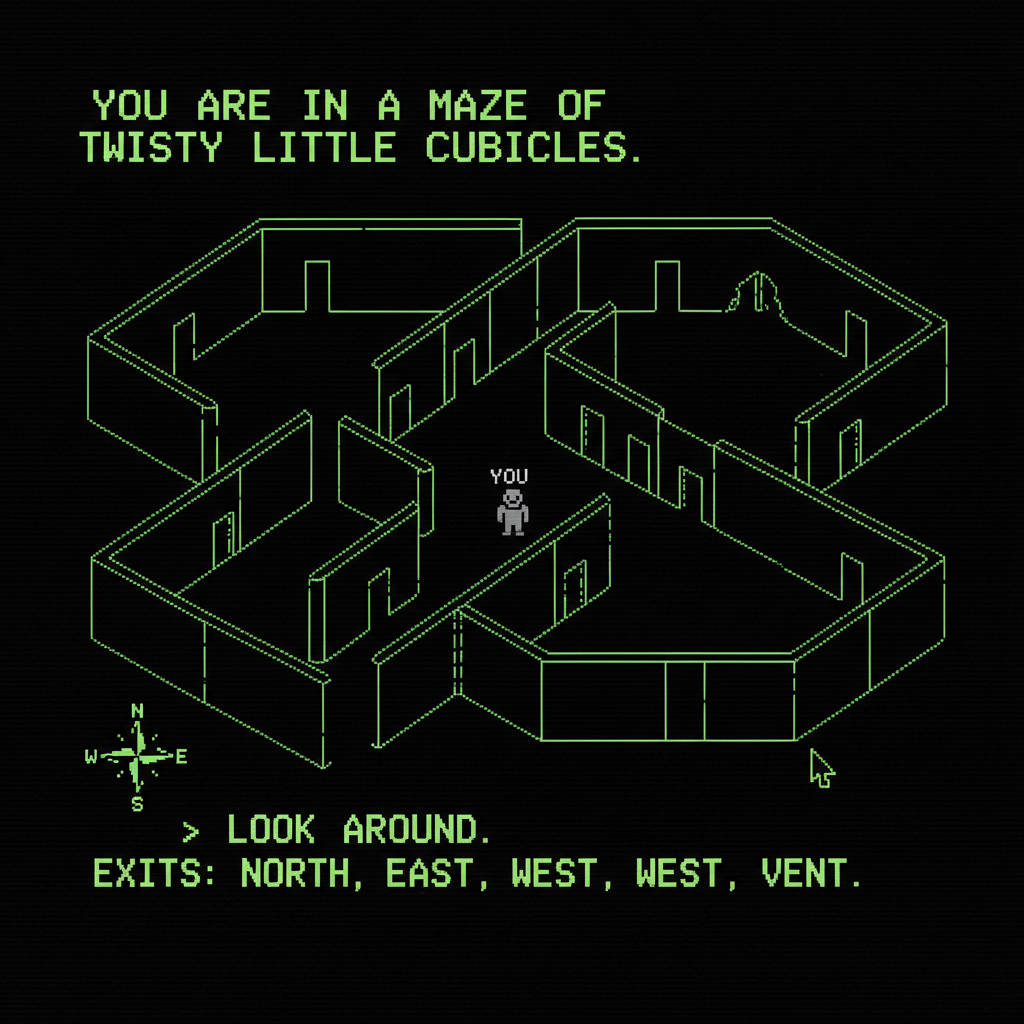
Day 13: A Maze of Twisty Little Cubicles

Useful Links

Concepts and Packages Demonstrated

NetworkX Matplotlib heapq Breadth-First Search (BFS)

Problem Intro

We’re in a maze of twisty little cubicles. We need to find the shortest path from a starting position to a destination. The maze is represented by a grid, where each cell is either an open space or a wall.

The input is a single number, which is our “favorite number”. This number is used in a formula to determine whether a given (x,y) coordinate is a wall or an open space.

The formula is: x*x + 3*x + 2*x*y + y + y*y + favorite_number. Then, find the binary representation of that value. If the number of 1s in the binary representation is even, it’s an open space. If it’s odd, it’s a wall.

For example, if the favorite number is 10, the top-left of the maze looks like this:

  0123456789
.#.####.##
..#..#...#
#....##...
###.#.###.
.##..#..#.
..##....#.
#...##.###

Part 1

What is the fewest number of steps required to move from (1,1) to (31,39)?

My strategy is to model the maze as a graph and then use a Breadth-First Search (BFS) algorithm to find the shortest path. I’ve chosen to use the networkx library for this, as it provides a simple way to create and work with graphs, and it has a built-in shortest path algorithm.

First, I created a Point2D class to represent coordinates. This class can generate its neighbors and check for equality.

The core of the solution is a BFS implementation:

Create a networkx graph g.
Use a set to keep track of explored points.
Use a heapq as a priority queue for points to visit.
Start at the START point, mark it as explored, and add it to the queue and the graph.
While the queue is not empty and the destination has not been reached: a. Pop a point from the queue. b. Get all its valid, unexplored neighbors. c. For each neighbor, add it to the graph, mark it as explored, and add it to the queue.

Once the BFS is complete (i.e., the destination is found or the queue is empty), I can use networkx.shortest_path(g, START, dest) to get the shortest path. The length of this path minus one is the number of steps.

Here’s the main part of the code:

import networkx as nx
import heapq

# ... (Point2D class and other setup)

def main():
    # ...
    
    # Part 1
    graph = nx.Graph()
    
    points_explored = set()
    points_explored.add(START)      # Mark our START as explored
    points_queue: list = [START]
    
    graph.add_node(START)
      
    while dest not in points_explored and points_queue:
        current_point = heapq.heappop(points_queue)
        
        valid_neighbours = [neighbour for neighbour in current_point.yield_neighbours() 
                                if is_open(neighbour) 
                                and neighbour not in points_explored 
                                and is_valid_coord(neighbour)]
        
        for neighbour in valid_neighbours:
            if neighbour not in points_explored:
                points_explored.add(neighbour)
                graph.add_node(neighbour)
                graph.add_edge(current_point, neighbour)
                heapq.heappush(points_queue, neighbour)
                
    solution_path = nx.shortest_path(graph, source=START, target=dest)
    logging.info(f"Steps required: {len(solution_path)-1}")

Part 2

How many distinct locations can be reached in at most 50 steps?

For this part, we can leverage the graph we built in Part 1. networkx provides a convenient function called nx.single_source_shortest_path(g, START, cutoff=50). This function returns a dictionary of all nodes that can be reached from the START node within the given cutoff distance. The length of this dictionary is our answer.

    # Part 2
    max_steps = 50
    
    paths = nx.single_source_shortest_path(graph, START, cutoff=max_steps)
    print(f"Destinations with no more than {max_steps} = {len(paths)}")

This is much more efficient than trying to calculate this manually.

Alternative Solution

I also implemented a pure BFS solution without using the networkx library. This solution builds a dictionary that maps each point to the path taken to reach it.

The logic is similar to the networkx solution, but instead of building a graph object, I manage the paths manually.

    # Part 1
    points_explored = set()
    paths_to_points: dict[Point2D, list[Point2D]] = {START: []}  # map each point to the path that gets to this point
    
    points_explored.add(START)      # Mark our START as explored
    points_queue: list = [START]
        
    while dest not in points_explored and points_queue:
        current_point = heapq.heappop(points_queue)
        
        valid_neighbours = [neighbour for neighbour in current_point.yield_neighbours() 
                                if is_open(neighbour) 
                                and neighbour not in points_explored 
                                and is_valid_coord(neighbour)]
        
        path_with_current = paths_to_points[current_point] + [current_point]        
        for neighbour in valid_neighbours:
            if neighbour in paths_to_points and len(paths_to_points[current_point]) <= len(path_with_current):
                continue    # Don't set the path if we already have a shorter path defined for this neighbour
            
            paths_to_points[neighbour] = path_with_current
            points_explored.add(neighbour)
            heapq.heappush(points_queue, neighbour)

For Part 2, I can filter the paths_to_points dictionary to include only the paths with a length less than or equal to 50.

    # Part 2
    max_steps = 50
    filtered_locations = dict(filter(lambda item: len(item[1]) <= max_steps, paths_to_points.items()))
    logging.info(f"Points we can reach in no more than {max_steps} = {len(filtered_locations)}")

Solution Comparison

Both solutions effectively solve the puzzle using a BFS approach.

NetworkX Solution: This approach is more concise and readable, as it abstracts away the details of the graph implementation. The networkx library is powerful and well-suited for this type of problem. However, it introduces an external dependency. For this puzzle, the performance is slightly slower than the pure BFS implementation, but still very fast.
Pure BFS Solution: This solution is more verbose but has no external dependencies (other than standard libraries). It gives more direct control over the pathfinding logic. In this case, it was marginally faster.

Conclusion: For this particular puzzle, the networkx solution is arguably better due to its clarity and simplicity. The minor performance difference is negligible. However, if performance were critical or if I wanted to avoid external libraries, the pure BFS implementation would be a solid choice.

Results

Here’s the output from the networkx solution:

Steps required: 92
Destinations with no more than 50 = 124
Execution time: 0.0038 seconds

And from the pure BFS solution:

Steps required: 92
Points we can reach in no more than 50 = 124
Execution time: 0.0030 seconds

‹›