Learning Python with Advent of Code Walkthroughs
Dazbo's Advent of Code solutions, written in Python
The Python Journey - Complex Numbers
Useful Links
Complex NumbersComplex Numbers in PythonMatplotlib
Page Contents
Introduction
Complex numbers are a mathematic concept. They are the combination of a real number (the kinds of numbers you’re used to working with every day), and a so-called imaginary number. Imaginary numbers, when squared, return a negative result. And this is why they’re imaginary! With real numbers, the result of any negative number multiplied by itself is always a positive number. And thus, it is impossible to have the square root of a negative number. And yet, this is the very definition of an imaginary number.
By convention, we say:
\(\sqrt{-1} = j\)
(Sometimes we use i instead of j.)
Whereas, with real numbers \( \sqrt{4} = 2 \), with imaginary numbers:
\[\begin{align} \sqrt{-4} = 2j \\ \sqrt{-25} = 5j \end{align}\]And so on.
And to conclude: a complex number is the combination of a real number and an imaginary number. For example:
\( 5 + 3j \)
In fact, the regular number 5 can be represented as a complex number! I.e. a regular number is a complex number that simply doesn’t have an imaginary component. E.g.
\( 5 + 0j \)
So What?
This mathematical definition is all well and good. But why should you care?
Well actually, for many practical applications of complex numbers in Python, you don’t need to know about any of the stuff above. You just need to know that:
Complex numbers are first class citizens in Python.
You can define them just as easily as any other variable type. E.g. \
my_complex_num = 5 + 3j
It is easy to add complex numbers
E.g.
num_a = 5 + 3j
num_b = 20 + 5j

num_c = num_a + num_b
print(num_c)
Output:
(25+8j)
They are useful for plotting two dimensional coordinates
Complex numbers are a really useful shorthand for working with x, y coordinates on a two dimensional graph. Think of the real numbers as the x axis, and the imaginary numbers as the y axis. When we do this, the resulting plot is known as an Argand diagram.
As a result, complex numbers can make it really convenient to do things like:
- Getting the horizontal (real) and vertical (imaginary) components of a vector.
- Adding and subtracting vectors.
- Calculating the magnitude of the vector (i.e. the hypotenuse).
# Define the points as complex numbers
point1 = complex(x1, y1)
point2 = complex(x2, y2)

# Calculate the difference between the two points
difference = point2 - point1

# Calculate the magnitude of the vector
distance = abs(difference)
- Calculating the angle of a vector.
# Calculate the difference (vector) between the two points
vector = point2 - point1

# Calculate the angle of the vector
angle_radians = cmath.phase(vector)
angle_degrees = math.degrees(angle_radians)
- Flipping, scaling and rotating vectors.
vector = point2 - point1

# Flip over the x-axis
flip_x = complex(vector.real, -vector.imag)
flip_y = complex(-vector.real, vector.imag)

# Rotate by theta degrees
theta = math.radians(degrees)  # Convert degrees to radians
rotation_factor = cmath.exp(1j * theta)
rotated_vector = vector * rotation_factor

# Scale by a factor
scale_factor = 2  # Example scaling factor
scaled_vector = vector * scale_factor
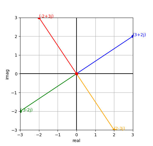
Just as a quick demo, here’s a visualisation using complex numbers and Matplotlib:
from matplotlib import pyplot as plt

def cw_rotate(z: complex, degrees: float) -> complex:
    """ Returns a new point, after rotating the supplied point about the origin,
    the specified number of degrees, clockwise. """
    # Note that complex number phase is expressed as a CCW angle to the real axis.
    # Thus, to rotate CW, we have to always take the supplied angle from 360.
    return z * 1j**((360-degrees)/90)

points: list[complex] = [] # store our points

POINT = 3+2j # starting point
print(POINT)
points.append(POINT)

for cw_angle in (90, 180, 270):
    rotated_point = cw_rotate(POINT, cw_angle)
    points.append(rotated_point)

fig, axes = plt.subplots()  # Create out axes
axes.set_aspect('equal') # set x and y to equal aspect
axes.grid(True) # add grid lines

# add lines at x=0, y=0
plt.axhline(0, color='black')
plt.axvline(0, color='black')

# set the limits and labels for each axis
all_x = [num.real for num in points]
all_y = [num.imag for num in points]
axes.set_xlim(min(all_x), max(all_x))
axes.set_ylim(min(all_y), max(all_y))
axes.set_xlabel("real")
axes.set_ylabel("imag")

colours = ['blue', 'orange', 'green', 'red']

# Iterate over each point and plot
for i, point in enumerate(points):
    # For this point, plot from origin to the point
    plt.plot([0, point.real], [0, point.imag], '-', marker='o', color=colours[i])

    # Add an annotation to the point.  We can do this one of two ways...
    # plt.text(point.real, point.imag, str(point))
    plt.annotate(str(point), (point.real, point.imag), color=colours[i])

plt.show()
The result is a plot that looks like this: